KEDE Forecasting

Introduction

Typically, project estimation methods and frameworks focus on factors such as task breakdown, resource allocation, past experience, or statistical models. By bringing the knowledge discovery process to the forefront, we're highlighting the importance of understanding the learning curve, problem-solving, and adaptation involved in software projects, and how these factors contribute to the overall completion time.

Emphasizing the role of knowledge discovery as part of software development projects in forecasting completion time provides a fresh perspective for project managers to consider when estimating and managing software projects.

We will be using Reference Class Forecasting (RCF) as a useful tool for improving the accuracy of software project estimates, as it relies on objective data from similar projects rather than relying solely on expert judgment or intuition.

By integrating the knowledge discovery process into RCF, you can create more nuanced and accurate project completion time forecasts, considering both historical data from similar projects and the unique learning and problem-solving aspects of your project.

The emphasis on the knowledge discovery process in forecasting completion time is a unique perspective that highlights the importance of learning, problem-solving, and adaptation in software projects. This perspective encourages project managers to consider the learning curve and the team's ability to acquire and apply new knowledge when estimating project completion times. You can think of it as a knowledge-centric approach to software project estimation and management, which is informed by various sources, such as agile methodologies, traditional project management approaches, math and empirical evidence from software development projects.

By focusing on the underlying knowledge discovery process and considering the learning and problem-solving aspects of software development projects, you can improve the accuracy of your completion time forecasts and better manage the project's timeline.

Reference Class Forecasting (RCF)

Reference Class Forecasting (RCF). Reference Class Forecasting is an estimation technique based on the idea of using historical data from similar projects, or a "reference class," to predict the outcomes of a current project. Developed by Daniel Kahneman and Amos Tversky as part of their work on decision-making and cognitive biases, RCF aims to reduce the influence of optimism bias and planning fallacy on project estimates[3].

Reference Class Forecasting (RCF) improves the accuracy of forecasts by taking an "outside view" of the project being forecasted. The outside view refers to the process of looking at the historical data of similar projects to create a more objective and reliable forecast for the current project. This approach contrasts with the "inside view," which is based on subjective expert judgment and is often influenced by optimism bias and the planning fallacy.

For many years, Bent Flyvbjerg has been a strong advocate for the use of Reference Class Forecasting to improve the accuracy of project estimates. He is well-known for his work on project management, particularly regarding cost overruns, schedule delays, and the planning fallacy in major infrastructure projects[4].

Here's an overview of how to apply Reference Class Forecasting to software project estimation:

Identify a suitable reference class: Find a set of similar completed software projects that can serve as a basis for comparison. These projects could share common complexity factors with your current project, such as requirements complexity, client type, team structure, technology expertise, domain expertise, and development process, as these factors affect project complexity which influences the knowledge discovery process. The class must be broad enough to be statistically meaningful but narrow enough to be comparable with the specific project.
Collect historical data: Gather data from the reference class on the key metric cumulative growth rate of knowledge discovered. This requires access to credible, empirical data for a sufﬁcient number of projects within the reference class to make statistically meaningful conclusions. Make sure the data is reliable and representative of the outcomes you want to predict.
Calculate the distribution: Analyze the historical data to determine the distribution of outcomes, such as completion time or cost, for the reference class. Additionally, analyze the impact of knowledge discovery aspects, such as learning curves and problem-solving efforts, on project outcomes.
Forecast project outcomes: Use the distribution derived from the reference class to forecast the likely outcomes for your current project. This may involve determining the percentile that corresponds to your project's characteristics and using it to predict completion time, cost, or other metrics. Incorporate the impact of knowledge discovery aspects to create a more informed completion time forecast.
Continuously update estimates: As your project progresses, collect new data and update your reference class. Refine your estimates by considering the ongoing knowledge discovery process and its impact on project outcomes. This will help you improve the accuracy of your forecasts.

Identify a suitable reference class

To implement Step 1, "Identify a suitable reference class" of Reference Class Forecasting (RCF), we need to establish the complexity of your current project and then identify a suitable reference class of projects that share comparable complexities.

We will utilize the knowledge-centric perspective on project complexity as explained here. By emphasizing the discovery and application of knowledge, this approach is necessary and natural for software projects. It better addresses the unique challenges inherent in software projects, leading to more accurate estimations and improved project outcomes.

Project complexity refers to the amount of knowledge that needs to be discovered by the team throughout the project lifecycle for the successful completion of the project.

The missing information can be broadly categorized into two types:

WHAT needs to be done (the objectives or requirements)
HOW to accomplish the WHAT (the processes, methods, and techniques to fulfill these requirements).

It's essential to note that the observed missing information is a subjective evaluation of the actual missing information. The same project could have different observed missing information for different observers, depending on their prior knowledge, understanding, and perspective. Thus, project complexity represents the gaps in understanding or information that the project team believes they lack and need to learn.

Project complexity refers to the amount of knowledge about "What" to produce and "How" to produce it.

It is essential to emphasize that our approach does not focus on selecting similar technologies, business domains, team structures, development processes, or client types. Instead, we concentrate on selecting projects with a similar level of ignorance, i.e., knowledge that needs to be discovered.

It is essential to emphasize that we concentrate on selecting projects with a similar level of ignorance, i.e., knowledge that needs to be discovered.

By doing so, we can use a project implemented with Java for a startup as a reference class when our new project is in C# for a bank. This knowledge-centric approach allows for more relevant comparisons and better predictions, as it focuses on the shared challenge of discovering new knowledge, regardless of the specific context or technology used.

We'll be following the steps outlined here. Thus you will gain a deeper understanding of your project's complexity and be better equipped to select a suitable reference class for RCF. This, in turn, will enable you to make more accurate forecasts and ensure a higher likelihood of project success.

You may have a portfolio of past project to pick a reference class from, but the projects may not be categorized based on the factors influencing project complexity we listed in the previous section. Don't worry - if you have the source code you can visualize the curves of the knowledge discovery process of your previous successful projects, as explained in the next section. Now you can pick a curve that matches the combinations of factors for your current project.

Collect historical data

In software development projects, the knowledge discovery process encompasses the learning, problem-solving, research, and collaboration activities undertaken by the project team. This process is an inherent property of the software development system.

To implement Step 2, "Collect historical data," of Reference Class Forecasting (RCF), we must adopt an outside view. We cannot delve into the inner workings of the software project's black box by becoming directly aware of the learning and problem-solving activities. Instead, we can gain insight into the likely learning and problem-solving activities that will occur throughout the project lifecycle by examining the cumulative growth of knowledge discovered in reference projects.

The cumulative growth of knowledge discovered is used in various domains. One such domain is scientometrics, which is the study of measuring and analyzing scientific literature and research activities. Measuring the growth of knowledge can be effectively applied to software development projects because it provides valuable insights into the learning and problem-solving activities that occur throughout the project. Employing this metric enables us to adopt an outside view of the project by analyzing the knowledge discovery process in similar past projects.

Below is a diagram of the growth of knowledge discovered in bits for a real project[1].

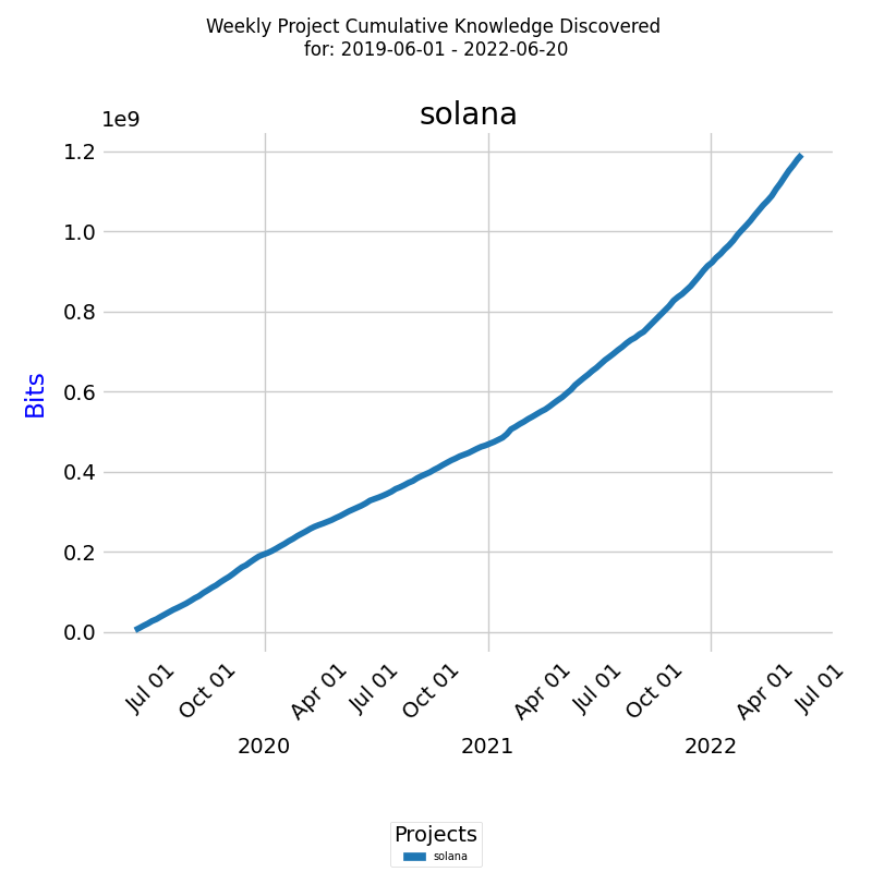
We can see the total growth of knowledge discovered in bits for the selected project and time period.

We also need to normalize the data to allow for a more meaningful comparison across reference class projects with varying magnitudes of knowledge discovered. Comparing raw values in bits may be misleading, as differences in scale can distort the true relative performance between projects.

To measure the normalized growth of knowledge discovered, we'll use the metric cumulative growth rate (CR) of knowledge discovered. The metric allows for:

taking an “outside view” on the development system that worked on the project
calculating delivery time
making sense from client's perspective

Employing this metric enables us to adopt an outside view of the project by analyzing the knowledge discovery process in similar past projects. The calculation of the metric is presented in the Appendix.

The diagram below shows the cumulative growth rate for the selected project for a specified period [1].

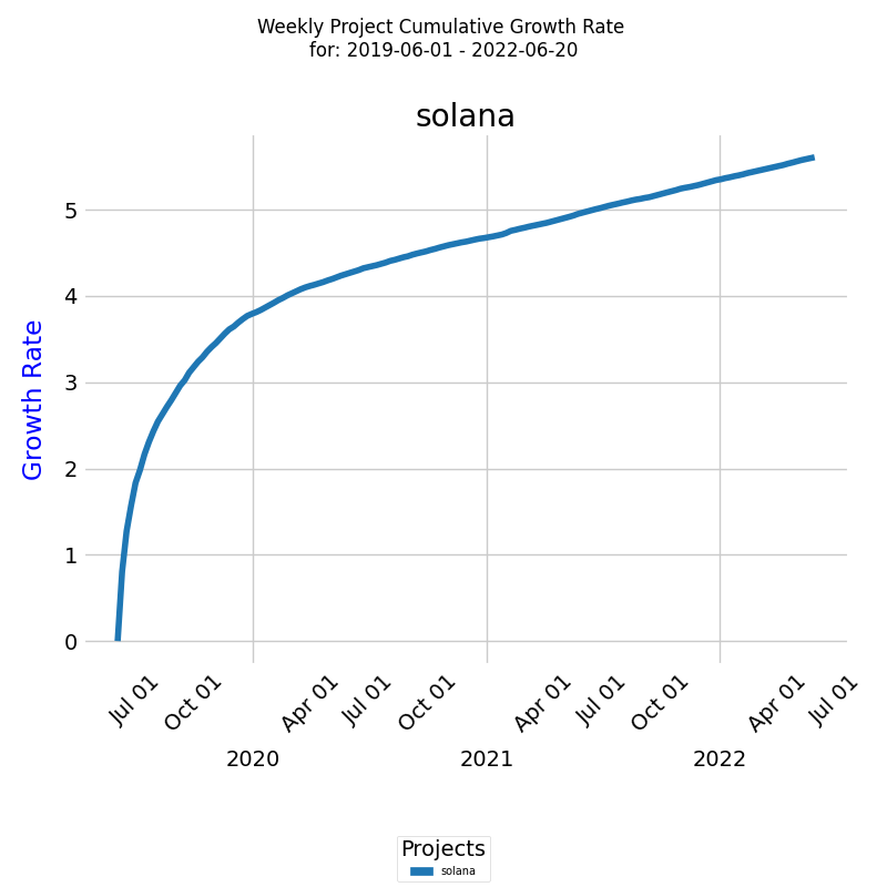
The x-axis represents the week dates, while the y-axis represents the cumulative growth rate. The line on the diagram represents the exponential cumulative growth rate during the selected period.

It's important to remember that the actual CR_T curve for a given project will depend on the unique combination of factors and their specific influence on the knowledge discovery process.

Establishing a probability distribution for the selected reference class

In order to implement Step 3 of Reference Class Forecasting (RCF), we will compare the CR_T time series for all projects that belong to the reference class. For comparing multiple Cumulative Return Time (CR_T) curves in terms of their similarity, we can use a statistical method and visual inspection.

Visual comparison

Visual comparison can provide a quick sense of the similarities or differences between the curves. By plotting them together on the same graph, we can observe how similar the curves are in terms of shape, peaks, and overall trend. If they appear similar, they belong to the same reference class.

The curve of CR_T for the combinations of factors listed here ould be influenced by the interactions among the factors and how they affect the rate of knowledge discovery.

The curve might vary significantly depending on the specific combination of factors, such as:

If a project has low requirements complexity, an experienced team, and high domain expertise, the CR_T curve might show a relatively stable and possibly lower growth rate, as the team will likely be able to discover the required knowledge more easily.
On the other hand, if a project has high requirements complexity, a less experienced team, and low domain expertise, the CR_T curve could display a steeper and more fluctuating growth rate, as the team may face more challenges and require more time to acquire the necessary knowledge.

However, this method is subjective and may not capture all the nuances of similarity or dissimilarity, especially when comparing many curves. For a more quantitative assessment, you can use statistical distance metrics.

Statistical method

Since we only have empirical data for each curve, we can use metrics based on the data points that do not require the analytical function of the curves. We're dealing with time series data where alignment and stretching are important factors.

We select Dynamic Time Warping (DTW) distance as our method. DTW measures the similarity between two time series by minimizing the distance between their points, allowing for non-linear time alignment. A smaller DTW distance indicates higher similarity. DTW is particularly useful when the curves have similar shapes but are misaligned in time or have different speeds.

We select Hierarchical Clustering as our clustering algorithm. This algorithm is a good choice for clustering curves. It does not assume any particular shape for the clusters, and it allows you to visualize the hierarchy of clusters to choose an appropriate number.

Note: Hierarchical clustering may not be the best method for separating a small number of curves, especially when the number of clusters is equal to the number of curves or when the distances between the curves are not significantly different.

In the diagram below, we have six project curves clustered into two clusters - blue and red:

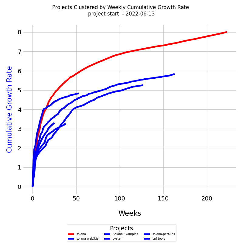
This diagram has six CR_T curves plotted, taking into account their different lengths in time units, and color the curves based on the clusters obtained from DTW distances.

If each curve has a different size in terms of time units, DTW can be applied to compare them, as it can handle time series of different lengths. However, ensure that the comparison is meaningful and that differences in time units do not lead to incorrect interpretations of similarity. When plotting the curves with different time units, we adjust the x-axis accordingly for each curve.

Preparing the distribution

By comparing the curves for all projects belonging to the reference class, we can see if they indeed belong to it. If one or two curves are significantly different from the rest, we can safely remove them from the reference class.

Eventually, we end up with data for all projects that belong to the reference class.

Forecasting Project Completion Time

Forecasting is inherently uncertain, as it involves making predictions about future events or trends. To better manage this uncertainty, we will be using a probabilistic forecasting approach that generates multiple scenarios to represent various possible outcomes.

The objective is to create an array of potential future scenarios for a project by considering the uncertainty in exponential growth rates. Each of these scenarios represents a unique way in which the project's knowledge discovery might unfold.

To forecast the total logarithmic growth rate for n developers for all time points in the interval [T+1, T+m], we will be using Prophet . This method, developed by Facebook, is a flexible and scalable forecasting model that can handle time series data with complex seasonality, trends, and irregular patterns.

To implement Step 4 of Reference Class Forecasting (RCF), we will follow these steps:

Gather data: Collect the CR_T time series for all projects that belong to the reference class.
Forecasting: Using each of the CR_T time series to forecast the completion time for your current project. We will make sure to consider uncertainty in the model predictions.
Histogram: After obtaining the completion time forecasts for your current project based on each CR_T time series, create a histogram of the completion time values to visualize the frequency distribution. The histogram will provide a visual representation of the likely completion times and their frequencies, allowing you to assess the overall distribution of possible completion times.

This method is a reasonable approach for forecasting the project completion time while accounting for the inherent uncertainty in the exponential growth rates. Just keep in mind that the actual project completion times may differ due to various factors not considered in the forecasting process.

Here is how the forecast may look like: on the forecast graph, the thick blue line represents the cumulative growth rate of the knowledge expected to be discovered for the successful delivery of the project. The x-axis displays the timeline of the new forecasted project, and the y-axis shows the cumulative growth of the knowledge to be discovered

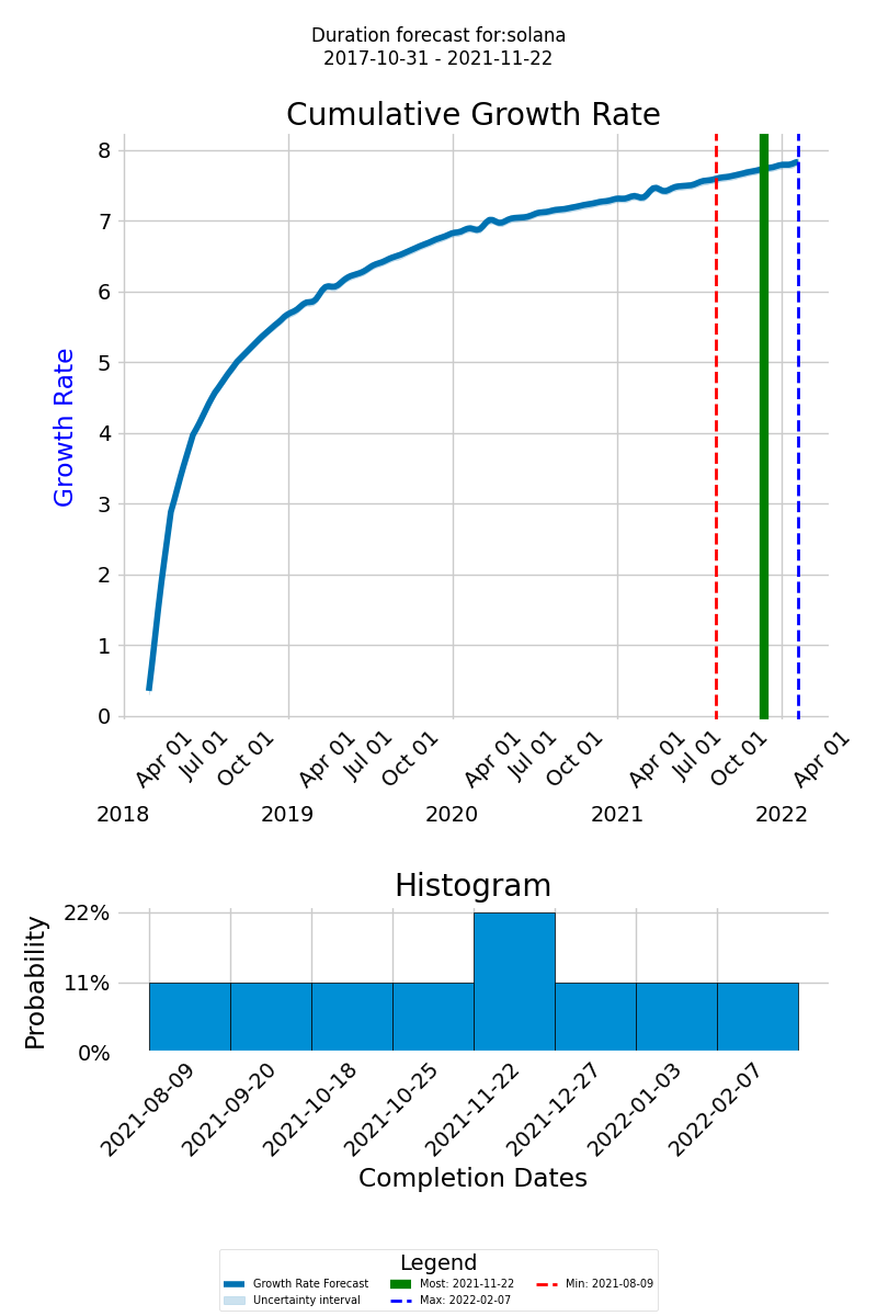
The green line represents the most likely completion date, the dashed red line indicates the earliest possible completion date, and the dashed blue line designates the latest possible completion date. This range of outcomes helps you prepare for different eventualities and plan your project more effectively.

The histogram of the completion dates is at the bottom of the diagram. Its purpose is to provide a visual representation of the likely completion dates and their probabilities, allowing you to assess the overall distribution of possible completion times.

Continuously updating the forecast

As your project progresses, collect new data and update your reference class to refine your forecast, by considering the ongoing knowledge discovery process and its impact on project outcomes.

Appendix

Exponential growth

The concept of cumulative growth rate is widely used in finance to measure the performance of investments or financial assets over time. For example, an investor might calculate the cumulative growth rate of a stock or a mutual fund over a certain period to determine the overall return on their investment. The cumulative growth rate can also be used to compare the performance of different investments over the same time period. Moreover, cumulative growth rate is also useful in analyzing economic growth or population growth over time.

In finance, compound returns cause exponential growth. The power of compounding is one of the most powerful forces in finance. This concept allows investors to create large sums with little initial capital. Savings accounts that carry a compound interest rate are common examples of exponential growth.

To calculate the cumulative growth rate we'll be using an exponential growth model. Exponential growth models describe a quantity that grows at a rate proportional to its current value. The general form of an exponential growth model is:

$y (t) = y (0) e^{k t}$

where y(t) is the value of the quantity at time t, y(0) is the initial value, k is the growth rate, and e is the base of the natural logarithm.

There are two cases - when the exponential growth rate over the interval from t=0 to t=T-1. is a constant and when it changes over time.

Constant exponential growth rate

To calculate the exponential growth rate of knowledge discovered Q, we can use the following general formula:

$R = \frac{d Q (t)}{Q (t)}$

The general formula calculates the exponential growth rate based on the ratio of the rate of change of knowledge discovered dQ/dt to the knowledge discovered Q at each time point.

If we know the initial knowledge discovered Q(0) and the exponential growth rate, we can calculate the knowledge discovered at a later time, such as Q(T), assuming the exponential growth rate remains constant over the given time interval.

To find the value of Q(T), we need to integrate this equation. For this purpose, we can use the following steps:

Rearrange the equation: dQ(t) / Q(t) = R
Integrate both sides with respect to time (t): ∫(dQ(t) / Q(t)) dt = ∫(R) dt
The integral of the left-hand side is the natural logarithm of Q(t): ln(Q(t)) = R * t + C
Solve for Q(t): Q(t) = e^(R * t + C)
Now, you can use the initial condition Q(0) to find the constant C:
Q(0) = e^(R * 0 + C) = e^C

C = ln(Q(0))

Finally, you can find Q(T) using the formula:

$Q_{T} = e^{R T + \ln (Q_{0})}$

This calculation assumes a constant exponential growth rate over the interval from t=0 to t=T-1.

Cumulative growth rate of knowledge discovered

When the exponential growth rate changes over time, we would need to know the function describing its change or have a time-series of exponential growth rates to calculate knowledge discovered Q(T).

In finance, the natural logarithm (ln) of the ratio between the future value and the current value of a financial asset is often used to calculate the exponential growth rate. This is referred to as the logarithmic or log return and measures the rate of exponential growth during a specific time period.

$R (t) = \ln (\frac{\sum_{i = 1}^{t + 1} Q (i)}{\sum_{i = 1}^{t} Q (i)})$

The log return R_t at a specific time step t represents the logarithm of the ratio of the sum of the knowledge acquired up to time t+1 to the sum of the knowledge acquired up to time t. The log return measures the relative growth in knowledge between two consecutive time steps, with higher values indicating faster growth.

The log return for a time period is the sum of the log returns of partitions of the time period. For example the log return for a year is the sum of the log returns of the days within the year. We will cal this cumulative growth rate because it is more proper for the context of knowledge management in projects.

The cumulative growth rate CR_T over the duration of the project up to time T is calculated using the formula:

$C R_{T} = \sum_{t = 0}^{T - 1} R (t)$

CR_T is the sum of the log returns R_t at each time step t from the beginning of the project (t=0) to the end of the project (t=T-1). CR_T represents the overall rate of knowledge growth in the project. The cumulative growth rate CR_T represents the proportionality constant for the growth of knowledge discovered H_T over time.

To calculate the total knowledge discovered Q_T at a given time T, we use the formula:

$Q_{T} = Q_{0} e^{C R_{T}}$

Here, H₀ represents the initial knowledge at the beginning of the project, and e^CR_T represents the exponential growth factor driven by the growth rate CR_T. The total knowledge discovered at time T is the product of the initial knowledge and the exponential growth factor.

Together, these three formulas provide a framework for quantifying and tracking the growth of knowledge in a project over time. By calculating the log returns R_t and cumulative growth rate CR_T, we can gain insights into the dynamics of knowledge discovery and make comparisons between different projects or strategies.

Using the cumulative growth rate (CR) instead of the time-series of knowledge discovered when comparing projects offers several advantages:

Normalization: CR is derived from the og returns (R), which inherently normalize the growth rates and allow for a more meaningful comparison across projects with varying magnitudes of knowledge discovered. Comparing raw H values may be misleading, as differences in scale can distort the true relative performance between projects.
Relative performance: CR captures the overall rate of knowledge discovery throughout the project duration, making it possible to evaluate the relative performance of different projects, strategies, teams, or methodologies. By comparing the cumulative growth rates, you can determine which project experienced a higher overall rate of knowledge growth. In contrast, comparing H values directly may not provide the same level of insight into relative performance, as it focuses on the absolute amount of knowledge discovered rather than the rate of growth.
Stability: CR is generally more stable and less susceptible to fluctuations due to random or transient events. By summing up all log returns (R) over the project duration, CR smooths out short-term variations and captures the overall trend of knowledge growth. This provides a more reliable basis for comparison between projects, as it minimizes the impact of noise or isolated events. Comparing H values directly may be more sensitive to such fluctuations, making it harder to discern underlying trends.
Simplicity: CR provides a single, summary metric that encapsulates the overall knowledge growth across the entire project lifecycle. This simplifies the comparison process by reducing the complexity of the data and allowing for a more straightforward interpretation of results. Comparing time-series of H values requires evaluating a multitude of data points, making it more challenging to draw meaningful conclusions.

Total exponential growth rate for N developers

Calculating the exponential growth rate R_t for each of the N developers and then summing it will not be an accurate representation of the total exponential growth rate. The reason for this is that exponential growth rates are not additive.

The correct approach to calculate the total exponential growth rate at each time point t for N developers, we first need to calculate the sum of knowledge discovered Q for all developers at each time point. Then, we will use the given formula:

$R (t) = \ln (\frac{\sum_{i = 1}^{t + 1} Q (i)}{\sum_{i = 1}^{t} Q (i)})$

to calculate the exponential growth rate R_t. By doing this, we take into account the combined effect of all developers on the system's knowledge growth.

Here's a step-by-step process:

Calculate the sum of knowledge discovered Q for all developers at each time point.
Calculate the exponential growth rate R_t.

Clustering algorithms

When dealing with curves that follow a logarithmic pattern, the choice of clustering algorithm can still be influenced by various factors such as the number of clusters, the noise in the data, and other domain-specific considerations.

Here are some popular clustering algorithms that might be suitable for your task

K-Means Clustering: K-Means is a popular and easy-to-implement clustering algorithm. Although it assumes that clusters are convex and isotropic (i.e., the same in all directions), it can still be effective in many real-world situations. If you know the approximate number of clusters, you could try K-Means.
Hierarchical Clustering: This algorithm is a good choice for clustering curves. It does not assume any particular shape for the clusters, and it allows you to visualize the hierarchy of clusters to choose an appropriate number.
Hierarchical clustering may not be the best method for separating a small number of curves, especially when the number of clusters is equal to the number of curves or when the distances between the curves are not significantly different.
Gaussian Mixture Model (GMM): A Gaussian Mixture Model is a probabilistic model that assumes that the data is generated from several Gaussian distributions. If the data fits this assumption, GMM might be a good choice.
DBSCAN: DBSCAN does not require the number of clusters to be specified and can find clusters of arbitrary shape, making it a good option for data that doesn't meet the assumptions of K-Means.

As with many machine learning tasks, the "best" algorithm may depend heavily on the specifics of your data and what exactly you want to achieve. Experimenting with different algorithms and validating the results using appropriate evaluation metrics will likely be necessary to find the optimal solution for your particular problem.

If the curves are logarithmic, using a distance metric that takes into account the underlying pattern may be more important than the choice of the clustering algorithm itself.

Works Cited

1. Solana

2. Armour, P.G. (2003). The Laws of Software Process, Auerbach

3. Lovallo, D., and Kahneman, D. (2003), "Delusions of Success: How Optimism Undermines Executives' Decisions", Harvard Business Review, July, 56-63.

4. Flyvbjerg, B. (2009), “Survival of the unﬁttest: why the worst infrastructure gets built and what we can do about it”, Oxford Review of Economic Policy, Vol. 25 No. 3, pp. 344-367.

5. Strode, Diane E. and Huff, Sid L., "A Taxonomy of Dependencies in Agile Software Development" (2012). ACIS 2012 Proceedings. 26. https://aisel.aisnet.org/acis2012/26

How to cite:

Bakardzhiev D.V. (2023) Forecasting software development projects. https://docs.kedehub.io/kede-manage/kede-manage/kede-forecasting.html

Forecasting software development projects

Related Articles