Knowledge Discovery Efficiency (KEDE) and Multi-scale Law of Requisite Variety
A Knowledge-centric approach
Introduction
Complex systems fail not because they lack effort, intelligence, or resources, but because their internal capacity to respond does not match the structure of the challenges they face. This mismatch is not always visible in aggregate measures of performance, productivity, or total capability. It often hides in how knowledge, coordination, and decision-making are distributed across different levels of detail.
Ashby’s Law of Requisite Variety formalized this insight by stating that a system can successfully regulate its environment only if it possesses at least as much variety as the disturbances it must counteract. In its classical form, the law treats variety as a single scalar quantity. Yet real environments—and real systems—are structured across multiple scales, from fine-grained local variations to large-scale coordinated patterns.
This article develops a knowledge-centric formulation of regulation that makes this structure explicit. We interpret regulation as a process of knowledge discovery: a staged reduction of uncertainty through selection, learning, and coordination. Missing knowledge is treated as measurable information, and successful regulation corresponds to closing this informational gap.
We show how to operationalize the Multi-Scale Law of Requisite Variety as a multi-scale knowledge-matching problem by defining a scale-dependent “knowledge gap” H(X|Y)n and its corresponding Knowledge-Discovery Efficiency (KEDE) profile. KEDE provides an operational way to quantify how efficiently a system converts prior knowledge into effective responses, both globally and across scales, making it possible to diagnose where regulation fails, where knowledge is missing, and why success at one scale cannot compensate for failure at another.
The Law of Requisite Variety
Given a set of elements, its variety is the number of elements that can be distinguished. Thus the set {g b c g g c } has a variety of 3 letters. Variety comprises any attribute of a system capable of multiple 'states' that can be made different or changed.
The Law of Requisite Variety, formulated by W. Ross Ashby states that[2]:
For a system to effectively regulate its environment, it must have at least as much variety as its environment
Ashby's Law is held true across the diverse disciplines of informatics, system design, cybernetics, communications systems and information systems.
Information-Theoretic Formulation
For many purposes the variety may more conveniently be measured by the logarithm of its value. If the logarithm is taken to base 2, the unit is the bit of information. In practice, we use the Shannon information entropy, denoted by H. For a quantifiable variable, entropy is just another measure of variance[1].
Without regulation, the entropy of the system is H(X). The presence of the regulator should ideally remove uncertainty from X. Thus, the difference between H(X) and H(X∣Y) represents how much uncertainty the regulator removes:
Here, I(D;R) is the mutual information or the channel capacity, representing how effectively the regulator Y reduces uncertainty in the regulated environment D. The conditional entropy H(D|R) measures the uncertainty remaining in X after considering the actions or states of regulator R.
- If H(X∣Y) is large, then after the regulator has acted or observed, significant uncertainty about the controlled environment remains. This indicates poor regulation or insufficient regulator variety.
- Conversely, if H(X∣Y) is low (ideally approaching zero), then the regulator effectively predicts or controls the states of the regulated environment D.
In other words, the conditional entropy of the controlled system given the regulator should be as small as possible ideally zero - implying perfect regulation.
The law of Requisite Variety says that Y 's capacity as a regulator cannot exceed Y 's capacity as a channel of communication. Thus, all acts of regulation can be related to the concepts of communication theory by noticing that the “disturbances” correspond to noise, and the “goal” is a message of zero entropy, because the target value E is unchanging.
Knowledge Discovery Process
Successful (essential) outcomes do not depend solely on the variety of responses available to a system; the system must also know which response to select for a given disturbance. Effective compensation of disturbances requires that the system possess the ability to map each disturbance to an appropriate response from its repertoire. This “system knowledge” can take various forms across different systems—for example, it may be encoded as a set of conditional rules of the form: if (perceived disturbance), then (response) [3]. The absence or incompleteness of such knowledge can be quantified using the conditional entropy H(Y|X), which captures the system’s ignorance about how to respond correctly to each disturbance D. In other words, H(R∣D) measures how much the system lacks the necessary knowledge to match responses to disturbances. H(Y|X) = 0 represents the case of no uncertainty or complete knowledge, where the action is completely determined by the disturbance. represents complete ignorance. This requirement may be called the law of requisite knowledge[3]. Mathematically, requisite knowledge can be expressed as:
In the absence of such system knowledge, the system would have to select responses, until eliminating all disturbances. Thus, merely increasing the response variety H(Y) is not sufficient; it must be complemented by a corresponding increase in selectivity, that is, reduction in H(Y|X) i.e. increasing knowledge.
We refer to the process of narrowing down and selecting the appropriate response from its set of alternative responses as the Knowledge Discovery Process.
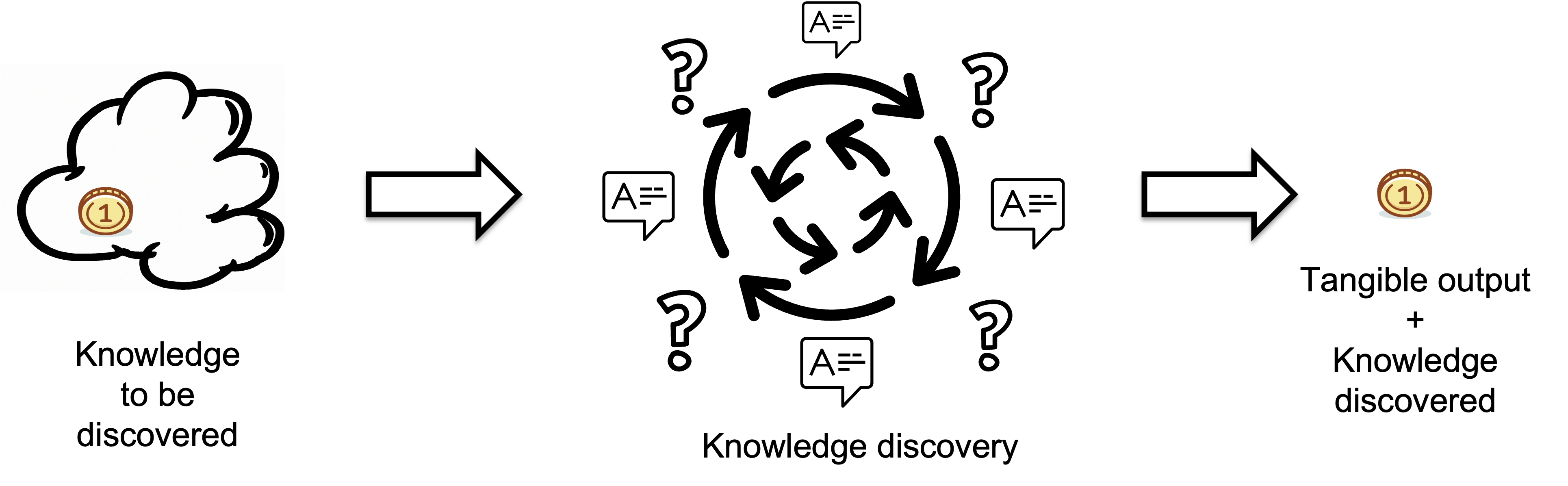
Inputs represent the knowledge a regulator lacks before starting a task i.e. the missing information or knowledge that needs to be discovered, which is measured in bits. The quality of the output is assumed to meet target standards.
The Knowledge Discovery Process is a multi-stage process of selection from a range of possibilities. At each stage, the system selects the most appropriate response based on the current state of its knowledge and the disturbances it faces.
Rather than a single act, selection is often a multi-stage process of selection from a range of possibilities[2]. Think of it as progressively reducing uncertainty at each stage — each stage reduces the complexity for the next stage.
Ashby’s Law of Requisite Variety states, for a staged selection process is[7]:
That is Ashby’s “requisite variety” restated: the sum of the bits removed by selection by every stage must at least equal the bits of uncertainty injected by the original range of possibilities (or by disturbances, in the regulation case).
Defining Knowledge to be Discovered
Knowledge to be Discovered H(X|Y) is the gap in internal variety that had to be compensated by selection.
Thus, the variety of the disturbances, is defined as the "required knowledge" or total unconditional missing information H(X), The regulators variety, or "prior knowledge" is defined as the mutual information I(X:Y), which equals the "requisite knowledge" we discussed earlier. The "knowledge to be discovered" is the conditional information H(X|Y) - what the regulator lacks about the task before starting it i.e. the gap in internal variety that had to be compensated by selection.
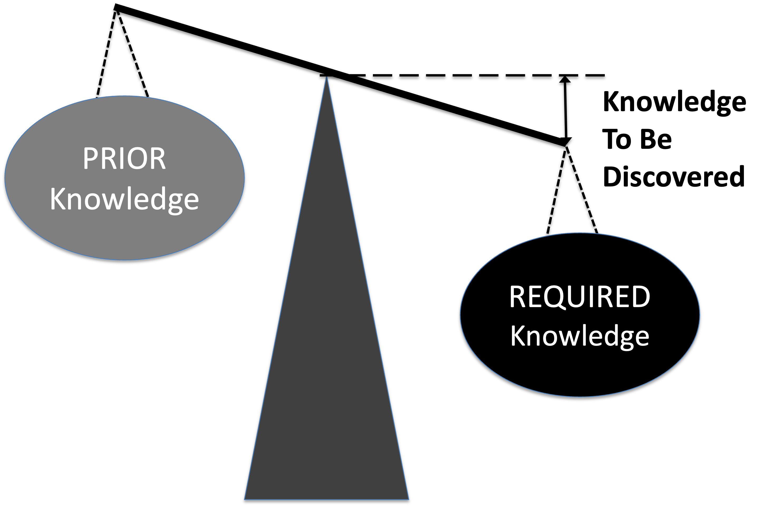
- Imagine a scale: on one side is the required knowledge and on the other is the prior knowledge.
- The gap between required and prior knowledge is the Knowledge to Be Discovered.
- They will be balanced if they are equal, implying that the knowledge to be discovered equals zero.
- When balanced, no further knowledge is needed; when imbalanced, knowledge acquisition is required.
Quantifying Knowledge To Be Discovered
We model the relationship between the knowledge to be discovered H(X∣Y) based on the observable outcomes E. We look at the case where the regulation was eventually successful. That is the knowledge discovery process closed the gap in internal variety that had to be compensated by selection i.e. eventually the knowledge to be discovered H(D|R) became 0.
The key idea is that the regulator's capacity to respond correctly is not static — it can change over time as the system learns and adapts.
We have a formula that allows us to calculate the average knowledge to be discovered by selection H(X|Y) for a time series {x} if we know the maximum output rate N, the total available time T and the actual output rate S[6].
(1)
If there is no knowledge to be discovered, i.e. there is no need to make selections at all, then S equals N and H is zero.
KEDE Definition
Here we generalize the Knowledge-Discovery Efficiency (KEDE) - scalar metric that quantifies how efficiently a system closes the gap between the variety demanded by its environment and the variety embodied in its prior knowledge[6].
To capture all of that we generalize the metric named KEDE. KEDE is an acronym for KnowledgE Xiscovery Efficiency. It is pronounced [ki:d].
We rearrange the formula (1) to emphasize that KEDE is a function of either H(X|Y) or S and N:
(2)
KEDE from (2) contains only quantities we can measure in practice. KEDE also satisfies all properties we defined earlier. it has a maximum value of 1 and minimum value of 0; it equals 0 when H is infinite; it equals 1 when H is zero;
KEDE effectively converts the knowledge to be discovered H(X|Y), which can range from 0 to infinity, into a bounded scale between 0 and 1. KEDE is inversely proportional to the knowledge discovered. The more prior knowledge was applied the more efficient a Knowledge Discovery process is. Conversely, when a lot of required knowledge is missing then the knowledge discovery is less efficient.
Due to its general definition KEDE can be used for comparisons between organizations in different contexts. For instance to compare hospitals with software development companies! That is possible as long as KEDE calculation is defined properly for each context. In what follows we will define KEDE calculation for the case of knowledge workers who produce textual content in general and computer source code in particular.
Anchoring KEDE to Natural Constraints
In our model, N is always the theoretical maximum output rate in an unconstrained environment, and S is the observed output rate under specific conditions over a given interval.
Both N and S can always be discretized—or “binned”—in a way that preserves the total information rate, regardless of whether the output arises from natural processes, human behavior, or machines. By choosing a bin width Δt small enough (e.g., milliseconds), the range of possible tangible outputs within each bin shrinks dramatically. This reduced range leads to less uncertainty in each bin, which compensates for the smaller time interval. Yet the ratio
remains an accurate measure of information rate.
Multi-scale Law of Requisite Variety
Interpreting Complexity Across Scales
Complexity is not an intrinsic, single-number property of a system. Rather,the information required to describe a system depends on the level of detail or scale at which the system is viewed. When we examine a system at very fine detail, we may see a large number of possible microstates; when we examine it at coarse scale, many microstate differences collapse into a smaller set of distinguishable macrostates. Complexity is therefore a function of scale, not a scalar[4].
To formalize this intuition, we consider systems composed of many components. If the components are people, then a task may require a certain (minimum) number of people acting together[4]. These components can be grouped into larger parts, and these partitions represent different scales by which the system may be described.
Any multi-scale structure can be represented by a sequence of nested partitions. The partition Pn contains exactly n parts, and the partitions must be nested. A nested sequence of partitions means each partition refines the previous one. Thus, each part in partition Pi is a subset of some part in partition Pi-1. This nesting ensures that as we move to finer scales (higher n), we gain more detail without losing the structure defined at coarser scales (lower n)[5].
This definition has strict properties:
- when n=1 then the system is one undivided whole (coarsest).
- when n=|X| then each component stands alone (finest).
- as n increases, the description becomes more detailed.
Scale is not:
- size of a group
- number of components in a part
- physical distance
- resolution
- granularity
- anything continuous
- the number of groups in a particular element of a nested partition sequence ,
- which defines how components of a set X are grouped,
- and includes all correlations exposed only because of the grouping at that level.
"Coarse-graining" means increasing the level of abstraction or simplification in a system, making the basic units larger and fewer, which reduces computational complexity but sacrifices detail. Fine scale means higher n, more groups, small group size, finer description. Large scale means lower n, fewer groups, large group size, coarser description. Fine-scale means independent behaviors. Large-scale means coordinated behaviors. Each latger scale reduces the number of distinct components by grouping them, thereby coarse-graining them. This hierarchical coarse-graining continues until we reach the coarsest scale, where all components are treated as a single unit.
To illustrate, consider a system with eight components. At the finest scale (scale 8), all eight components are distinct and independent. At scale 4, we group the components into pairs, yielding four coarse-grained units. At scale 2, we further group them into sets of four, resulting in two larger units. At scale 1, all components are combined into a single unit.
| Scale | Description | Components | |||||||
|---|---|---|---|---|---|---|---|---|---|
| 1 | coarsest | ||||||||
| 2 | further coarse-graining | ||||||||
| 4 | coarse-grained | ||||||||
| 8 | fine-grained | ||||||||
This notion of scale is distinct from the amount of variety (complexity) available at that scale. Given a nested partition sequence P of a system X at scale n , captures the total (potentially overlapping) information of the system parts when described through the partition Pn. Note that is the average amount of information necessary to describe one of the n parts[5].
The complexity profile at scale n of a system X viewed through a nested partition sequence P, is with the convention that . The complexity profile assigns a particular amount of information to the of a system X at each scale n. For where . The complexity at each scale measures the amount of additional information that becomes available when different parts of the system are considered separately[5].
This multi-scale view reveals deep structural constraints:
- At fine scales, complexity reflects the variety of individual components..
- At intermediate scales, complexity reflects partially redundant or partially coordinated behaviors.
- At large scales, complexity reflects coherent, system-level patterns that require many components to act in concert.
At fine scales, descriptions capture the variety of individual components; at larger scales, they capture the structured behaviors that emerge only when components act together. With coarse-graining at larger scales, you lose fine-grained distinctions, so the information cannot increase. it can only stay the same or decrease.
The scale-dependent framework rests on three structural steps:[5]:
- Partition the system into components and define how these components may be grouped at different scales.
- Construct a nested sequence of partitions, ensuring that each coarser partition is a grouping of the finer one.
- Measure complexity at each partition level by quantifying how much information remains after coarse-graining.
Through this construction, the complexity profile makes visible where a system’s information resides—whether predominantly at fine scales, at intermediate scales, or in large-scale coordinated behaviors.
The complexity profile also obeys a sum rule: Because the complexity at each scale measures the amount of additional information present when different parts of the system are considered separately, the sum of the complexity across all the scales will simply equal the total information present in the system when each component is considered independently of the rest[5].
The sum rule is a structural conservation law for descriptions of a single system. It ensures that information is only redistributed across scales, but not created or destroyed. This reflects a fundamental tradeoff: large-scale structure can exist only if small-scale degrees of freedom are constrained[5].
Generalizing Ashby to a Multi-Scale Setting
Ashby's classical Law of Requisite Variety states that a regulatory system must possess at least as much variety as the environmental conditions that require distinct responses. In other words, the conditional entropy of the controlled system X given the regulator Y should be as small as possible ideally zero - implying perfect regulation.
Consider two individuals who cannot coordinate. At a fine scale, they have more than enough behavioral variety as each person can act independently. But at the larger scale required to move a couch, they lack the necessary coordinated variety. Classical Ashby deems the system “sufficient,” but in practice it fails. The limitation is one of scale.
This motivates the Multi-Scale Law of Requisite Variety[4]:
For a system to effectively regulate its environment, its complexity must equal or exceed the environment's complexity at every scale.
To make this statement precise, the system and environment are each represented as a set of components equipped with corresponding nested partitions. At each scale n, the conditional entropy: , quantifies the missing information about the environment's state X at scale n given the knowledge of the system Y at scale n. Note: The parentheses refer to the same entropy measure applied to the same underlying variables. The subscript n refers to the scale at which the description is evaluated, not a new random variable. Thta is because H(X|Y) is a function of the joint distribution of X and Y, which can be analyzed at different scales using the nested partitions defined earlier. The distributions X and Y never change. Only the description changes with scale.
If this coarse-grained conditional entropy is zero: at scale n, then the system Y can fully distinguish all environmental states at that scale i.e. it perfectly regulates the environment X at that scale. If it is greater than zero, some information about X at scale n is missing from Y, indicating imperfect regulation at that scale.
This is the multi-scale operational version of Ashby's Law of Requisite Variety.
But computing conditional entropy requires knowing the joint distribution p(x,y). In many practical situations, this distribution is unknown or difficult to estimate. We typically know:
- what the environment does on its own (its complexity at various scales)
- what the system does on its own (its complexity at various scales)
Using the complexity profile at scale n, we compute complexity as a function of scale. When the system matches the environment — meaning each system component has a distinct response for each environmental condition relevant to it—the following necessary condition must hold:
and if at any scale , the system cannot fully regulate the environment, where and are the scale-dependent complexities of the system and environment at scale n, respectively.
Thus, a system cannot “add” large-scale capability without sacrificing some small-scale variety. The multi-scale law requires that the distribution of complexity across scales — not merely its total amount — must be appropriate for the task or environment.
This result is formalized in Theorem 1 of [5], which proves that if is even possible under some joint distribution of X and Y, then the inequality holds for every possible nested partition sequence, i.e. for every admissible way of defining scales. It also extends to every subset of components (Corollary 1), ensuring that not only the system as a whole but every subsystem must be at least as complex as the corresponding part of the environment.
Thus, is a necessary condition for . Conversely, if at any scale , then zero conditional entropy is impossible, meaning the system can never fully distinguish environmental states at that scale — indicating that the system cannot fully regulate the environment.
In summary:
- The complexity profiles and tell us whether it is possible for the system Y to distinguish environmental states X at scale n, without knowing the joint distribution. Thus, they measure capacity i.e. how much information is available at each scale.
- The conditional entropy tells us whether the system Y actually distinguishes environmental states X at scale n. Thus, it measures performance i.e. how much information is actually utilized at each scale.
The complexity profile has a sum rule because it measures conserved internal information. Conditional entropy has no sum rule because it measures relational uncertainty, which is not conserved across scales. Coarse-graining can make conditional entropy decrease, increase, vanish, or appear. Correlations with the environment can disappear at some scales while appearing at others This distinction is absolutely central to the multi-scale law of requisite variety. Failure to regulate at one scale cannot be compensated by success at another. If conditional entropy did obey a sum rule, then:
- If a system perfectly regulated its environment at some scales (zero conditional entropy), it would have to be less effective at other scales (higher conditional entropy) to conserve total conditional entropy.
- This would imply a tradeoff where excelling at regulation in one area necessitates failure in another, which contradicts the goal of effective regulation across all scales.
Implications
The multi-scale formulation strengthens Ashby’s original insight. A system is not effective simply because it has high total variety; it must have variety in the right places. A regulatory system, an organization, or a biological organism must align its complexity profile with the demands of its environment:
- granular variety where fine responsiveness is needed,
- coordinated large-scale complexity where collective action or coherent strategy is required,
- and appropriate structure at the intermediate scales where patterns of interaction matter.
By making scale explicit, the multi-scale law provides a precise mathematical criterion for diagnosing mismatches between systems and environments—showing when regulation or control is impossible, regardless of mechanism.
How KEDE operationalizes the Multi-Scale Law of Requisite Variety
The Multi-Scale Law of Requisite Variety provides a necessary condition for effective regulation: a system must possess sufficient complexity to match its environment at every relevant scale. However, the law by itself is structural — it tells us whether regulation is possible, not how well a real system is performing or how large the remaining knowledge gap is at each scale.
KEDE provides the missing operational layer.
At each scale n, the conditional entropy measures the remaining uncertainty about the environment after accounting for the system’s knowledge at that same scale.
This quantity is the scale-specific violation (or satisfaction) of Ashby’s requirement: if it is zero, requisite variety is met at that scale; if it is non-zero, regulation is structurally incomplete at that scale.
Using the observable output rates, we can compute this scale-dependent knowledge gap directly by applying the formula (1):
(3)
- N(n) is the maximum achievable output rate at scale n under unconstrained knowledge,
- S(n) is the actual output rate at scale n given the system's current knowledge.
To make this result comparable, bounded, and operational, we define the KEDE profile at scale n as:
(4)
KEDE(n) is therefore not an auxiliary metric, but the direct operational expression of multi-scale requisite variety:
- If at any scale n, KEDE(n) is low, the system lacks sufficient knowledge to handle the environment at that scale, even if it might look “fine” at others.
- If KEDE(n) = 1, then the knowledge gap is 0 at that scale i.e. the system fully satisfies Ashby’s Law at scale n,.
So at each scale, KEDE(n) is the fraction of the “potential complexity” the system has actually learned to tame. For a system to be effective, KEDE(n) must be 1 across all relevant scales, indicating that the system possesses adequate knowledge to manage the environment’s complexity at every level.
In other words:
- The complexity profile tells us how much environmental complexity exists and at which scales.
- KEDE(n) tells you how well a system knowledge matches that complexity at each scale.
Viewed across all scales, the KEDE profile functions as a multi-scale knowledge-gap tomography: it reveals precisely where a system’s internal knowledge and coordination are insufficient, even when aggregate performance appears acceptable.
Crucially, this makes explicit a core implication of the Multi-Scale Law: failure to satisfy requisite variety at one scale cannot be compensated by success at another. A system may appear efficient globally while remaining fundamentally incapable of regulation at specific scales where coordinated behavior or fine-grained responsiveness is required.
In this sense, KEDE does not merely fit into the multi-scale framework but it operationalizes it. The Multi-Scale Law defines what must be true for regulation to be possible; KEDE measures how close a real system is to meeting that requirement, scale by scale.
How to cite:
Bakardzhiev D.V. (2025) Knowledge Discovery Efficiency (KEDE) and Multi-scale Law of Requisite Variety https://docs.kedehub.io/knowledge-centric-research/kede-multi-scale-law-requisite-variety.html
Works Cited
1. Shannon, C. E. (1948). A Mathematical Theory of Communication. Bell System Technical Journal. 1948;27(3):379-423. doi:10.1002/j.1538-7305.1948.tb01338.x
2. Ashby, W.R. (1956) An Introduction to Cybernetics; Chapman & Hall, .
3. Heylighen, F., & Joslyn, C. (2001). Cybernetics and Second Order Cybernetics. In R. A. Meyers (Ed.), Encyclopedia of Physical Science and Technology, Eighteen-Volume Set, Third Edition (pp. 155-170). Academia Press. http://pespmc1.vub.ac.be/Papers/Cybernetics-EPST.pdf
4. Yaneer Bar-Yam.(2004) Multiscale variety in complex systems. Complexity, 9(4):37{45,
5. Siegenfeld, A.F.; Bar-Yam, Y. (2022) A Formal Definition of Scale-dependent Complexity and the Multi-scale Law of Requisite Variety. arXiv 2022, arXiv:2206.04896
6. Bakardzhiev, D., Vitanov, N.K. (2025). KEDE (KnowledgE Discovery Efficiency): A Measure for Quantification of the Productivity of Knowledge Workers. In: Georgiev, I., Kostadinov, H., Lilkova, E. (eds) Advanced Computing in Industrial Mathematics. BGSIAM 2022. Studies in Computational Intelligence, vol 641. Springer, Cham. https://doi.org/10.1007/978-3-031-76786-9_3
7. Bakardzhiev D.V. (2025) Knowledge Discovery Efficiency (KEDE) and Ashby's Law https://docs.kedehub.io/knowledge-centric-research/kede-ashbys-law.html
Getting started


