Knowledge Discovery Efficiency (KEDE) and Ashby's Law of Requisite Variety

Abstract

We address Real-world applications of Ashby's Law by adopting Ashby's strict black-box perspective: only external behaviour is observable. First we define the multi-staged selection process of narrowing down and selecting the appropriate response from the set of alternative responses as the Knowledge Discovery Process. We then establish H(X|Y) as the knowledge to be discovered, which is the gap in internal variety that had to be compensated by selection. This quantifies how much disorder the regulator still permits and, conversely, how close the system comes to meeting Ashby's requisite-variety condition. In information-theoretic terms, perfect regulation requires H(X|Y) = 0. Then we quantify the knowledge to be discovered H(X|Y) based on the observable outcomes. Building on this result, we generalize Knowledge-Discovery Efficiency (KEDE) - scalar metric that quantifies how efficiently a system closes the gap between the variety demanded by its environment and the variety embodied in its prior knowledge. KEDE operationalises requisite variety when internal mechanisms remain opaque, offering a diagnostic tool for evaluating whether biological, artificial, or organisational systems absorb environmental complexity at a rate sufficient for effective regulation. Finally we present applications of KEDE in diverse domains, including typing the longest English word, measuring software development, testing intelligence, basketball game, assembling furniture, and speed of light in medium.

Introduction

The Law of Requisite Variety, formulated by W. Ross Ashby, states that for a system to effectively regulate its environment, it must have at least as much variety/complexity as its environment[1]. This principle is foundational in disciplines such as cybernetics, control theory, and machine learning.

The concept of requisite variety has since been applied across diverse domains, including organizational theory, ecology, and information systems. It underscores the necessity for systems to adapt to environmental complexity in order to maintain stability and achieve intended outcomes.

Real-world attempts to apply Ashby's Law of Requisite Variety face three persistent obstacles. (i) Combinatorial explosion: enumerating all relevant states of a system and its environment quickly becomes intractable, especially when hidden or unmeasured variables are present. (ii) Dual control dilemma: a regulator must simultaneously amplify its own control variety and attenuate external variety—an optimization that is delicate in multiscale, hierarchical, and time-varying settings such as digital ecosystems or military command structures. (iii) Resource constraints: limited data, computational power, and organisational capacity often preclude sophisticated control architectures. Existing remedies—markup-language state catalogues, iterative multidimensional sampling, and distributed self-organising controllers—mitigate but do not eliminate these limitations.

In section 2, we conduct a literature review of the primary challenges in applying Ashby's Law to real-world systems and propose a black-box solution: treating the system as a black box, observing the probability of successful outcomes to disturbances, and estimating the gap in its internal variety from that. In section 3, we present the Law of Requisite Variety in both its set-based formulation—covering the Table of Outcomes, requisite variety, goal revision, and behavioral rework—and its information-theoretic formulation, covering entropy, probabilistic success, residual variety bounds, response-equivalence, and the regulator's learned law of action. We conclude section 3 by introducing Knowledge To Be Discovered as the conditional entropy H(X|Y) that remains after available disturbance information is known. In section 4, we establish the Knowledge Discovery Process as the staged reduction of Knowledge To Be Discovered. We develop this in three layers: a set-based formulation of staged selection covering episodes, closures, and rule regulation; an information-theoretic formulation introducing the expected staged reduction of H(X|Y), action units, and response-class commitment; and learning across episodes, including comparable episodes, the learning axiom, and the posterior-becomes-prior rule. We also develop the operational ledger and the knowledge ledger, together with their window-level accounting measures and a three-loop feedback reading of all revisions. In section 5, we show how to quantify Knowledge To Be Discovered from observable outcomes alone, deriving the operational one-bit effective-depth estimator. and its relationship to the latent entropy. In section 6, we generalize the Knowledge-Discovery Efficiency (KEDE)—a scalar metric in [0,1] that quantifies how efficiently a system closes the gap between the variety demanded by its environment and the variety embodied in its prior knowledge. Finally, in section 7, we explore applications of KEDE across diverse domains including manual assembly, typing, software development, intelligence testing, sports performance, industrial assembly lines, and the speed of light in a medium, demonstrating its utility as a unified diagnostic tool for evaluating system performance and adaptability.

Core challenges in applying Ashby's Law to real systems

We conducted a literature review aimed at identifying the primary challenges and limitations associated with applying Ashby's Law in real-world systems.

A central challenge that emerges is the measurement of variety. In most of the reviewed literature, the concept of variety is either poorly defined or not explicitly measured, resulting in ambiguity and potential misinterpretation of the law's implications. Key obstacles to effective measurement include:

The direct measurement of variety is fundamentally incomputable for all but the simplest systems [14].
Hidden variables introduce uncertainty and complicate measurement efforts [15].
Trade-offs often arise between variety at different scales [16].
A combinatorial explosion occurs when attempting to enumerate all possible system states [15,16].
Resource limitations constrain the feasibility of comprehensive measurement [20].
Environmental complexity is frequently “unknowable,” preventing complete assessment [25].
Most studies lack explicit or standardized methods for quantifying variety [14,17'-20,25,27].
Existing approaches often lack rigorous quantitative validation [17].

Several measurement methods have been proposed, including:

Markup language-based variety estimation [18],
Iterative sampling techniques [21],
Entropy and determinism metrics to evaluate communication complexity, where greater variety was correlated with improved effectiveness [22],
Social network and cluster analysis to assess resilience [23], and
Multiple Correspondence Analysis (MCA) for capturing organizational complexity [24].

In addition, a subset of studies estimate variety through observed performance rather than structural attributes. Notable examples include:

Communication-based performance measures, employing determinism metrics to evaluate repeatable patterns in team behavior [22];
Team performance assessments, using task-based surveys to evaluate an organization's risk-handling capabilities [23];
Leadership behavior analysis, based on actual behavioral responses to simulated scenarios [26]; and
Relative performance comparisons, assessing organizational effectiveness across contexts using perception-based rather than absolute metrics [14].

While these performance-based approaches provide practical insights, they often rely on subjective or indirect indicators of variety, which may introduce biases and limit their generalizability. For example, performance outcomes may fail to account for hidden variables or the underlying complexity of the system [15]. Moreover, these approaches remain underrepresented in the literature, where structural and theoretical analyses still dominate.

In summary, although numerous methods for measuring variety have been proposed, no single comprehensive or universally accepted solution has emerged. Quantification remains a persistent challenge in the application of Ashby's Law to complex real-world systems.

Solution

These challenges significantly hinder the practical application of Ashby's Law. Whether considering a human, an AI model, or an organization, we are typically limited to observing external behavior rather than internal mechanisms—unless we are able to "open the box."

Ashby himself emphasized that all real systems can be considered black boxes. He argued that while black boxes mimic the behavior of real objects, in practice, real objects are black boxes: we have always interacted with systems whose internal workings are, to some extent, unknown.

This leads to what Ashby termed the black box identification approach [2], which involves:

Perturbing the system by applying external disturbances,
Measuring the system's responses to these perturbations, and
Inferring the internal variety or capacity from the observed input-outcome relationships.

In most practical scenarios, we are only able to observe the outcomes of a system. These observable outcomes can be used to infer bounds on the system's internal variety—specifically, the extent of variety it must possess or lack in order to exhibit the observed behavior.

We propose such an approach: to treat the system as a black box, observe the probability of successful outcomes to disturbances, and estimate the gap in its internal variety based on that. Let E denote the event that the system gives an response to disturbance D, and let R be the regulator's action. In information-theoretic terms, perfect regulation requires H(R|D) = 0[31]. Using our novel information-theoretic estimator, empirical estimates of P(E=1) are used to quantify H(R|D) in bits of information. This quantifies how much disorder the regulator still permits and, conversely, how close the system comes to meeting Ashby's requisite-variety condition.

The Law of Requisite Variety

For a system to effectively regulate its environment, it must have at least as much variety as its environment.

Set-based formulation

Regulation achieves a goal by selecting responses against disturbances.

$E = (E_{1}, \dots, E_{n})$ is the essential-variable vector. The essential variables $E_{1}, \dots, E_{n}$ are the goal-relevant state components. $E_{i}$ is the value set of $E_{i}$ . The essential variables define the dimensions; their value sets define the coordinate domains of the essential-variable space $E = E_{1} \times E_{2} \times ... \times E_{n}$ , which is the set of all possible combinations of their values[29].

An essential state $e \in E$ is one particular point in the essential-variable space, i.e. a tuple of values of these dimensions, e.g. $e = (36.8 ° C, 92 mg / dL, \dots)$ .

It is assumed that the goal has already been determined: the acceptable essential states are given by an acceptable region $η \subseteq E$ in the essential-variable space. Thus, the goal is a region in a multidimensional essential-variable space $E$ .

Let D, R, and Z denote, respectively, the disturbance variable, regulatory-response variable, and outcome variable. Let their corresponding sets of possible values be $D$ , $R$ , and $Z$ . Thus $d \in D$ , $r \in R$ , and $z \in Z$ are particular values.

In the general case, the outcome-value space may itself be multidimensional. Let $Z = (Z_{1}, \dots, Z_{m})$ be the outcome-variable vector. The outcome variables $Z_{1}, \dots, Z_{m}$ are the components used to describe the concrete or functional result produced by a disturbance-response pair. $Z_{j}$ is the value set of $Z_{j}$ . Thus the outcome-value space is $Z = Z_{1} \times Z_{2} \times ... \times Z_{m}$ .

An outcome-value $z \in Z$ is one particular point in the outcome-value space. In the multidimensional case, it has the form $z = (z_{1}, \dots, z_{m})$ . In the Appendix we have an example of a typing task, where an outcome-value may record both the intended target position and the typed symbol: $z = (p, a)$ .

The number of outcome dimensions m need not equal the number of essential-variable dimensions n. The outcome-value space $Z$ describes the result produced by the system, while the essential-variable space $E$ describes the goal-relevant state used to judge that result. The mapping from outcomes to essential-variable values will be introduced below.

The scalar outcome-value case is recovered when $m = 1$ . In that special case, each outcome-value may be treated as an unstructured value. More generally, each table cell still contains one outcome-value, but that outcome-value may itself be internally structured as a tuple.

We use roman $E$ for the essential-variable vector and script $E$ for its value space. Likewise, we use roman $Z$ for the outcome-variable vector and script $Z$ for its value space.

The Table of Outcomes is the map

T : D \times R \to Z

so that for each disturbance-value $d$ and response-value $r$ , the value $T (d, r)$ is the outcome-value $z \in Z$ .

Thus the table T is two-dimensional in its indexing by disturbance-response pairs (d,r), while each cell-entry may be a scalar outcome-value or a structured outcome-vector. The scalar-outcome case is recovered when $Z = Z_{1}$ .

T		R
T		r₁	r₂	r₃	...
D	d₁	z₁₁	z₁₂	z₁₃	...
	d₂	z₂₁	z₂₂	z₂₃	...
	d₃	z₃₁	z₃₂	z₃₃	...
	d₄	z₄₁	z₄₂	z₄₃	...
	...	...	...	...	...

Two distinct disturbance-response pairs may yield the same outcome-value:

T (d_{1}, r_{1}) = T (d_{2}, r_{2}) = z

This means that repetition belongs to the mapping T, not to the set $Z$ . A set contains each of its elements only once. So one should not say that $Z$ contains repeated values. What repeats is the same outcome-value appearing as the image of multiple table-cells.

Correspondence between outcome-values and essential-variable values. The “outcomes” in the Table of Outcomes are simple outcome-values, without any implication of desirability. An outcome-value $z \in Z$ is a concrete or functional result of a disturbance-response pair. An essential-variable value $e \in E$ is the goal-relevant state description used to judge whether the result falls inside or outside the acceptable region.

The correspondence between outcome-values and essential-variable values is therefore not automatic. It is part of the modeling frame of the regulatory problem. To use a function from outcomes to essential-variable values, the outcome-description must be specified at a level of detail sufficient to determine the relevant essential-variable value. In this article we assume that this has been done. Thus each outcome-value under the adopted description has a determinate associated essential-variable value.

φ : Z \to E

so that $φ (z) = e$ . This means that the function $φ$ is a modeling map from the outcome-description used in the table to the essential-variable description used for regulation. It should not be read as saying that every possible description of an outcome would automatically determine an essential-variable value. If the outcome-description were too coarse to determine the relevant essential-variable value, then $φ$ would have to be replaced by a relation, a refinement of $Z$ , or a probabilistic mapping.

The reduced, bijective, and many-to-one cases discussed below are therefore not alternatives to this modeling assumption. They are different ways in which the adopted outcome-description may correspond to the essential-variable description. In the reduced case, outcome-values already are essential-variable values. In the bijective case, outcome-values and essential-variable values are distinct descriptions but correspond one-for-one. In the many-to-one case, several finer-grained outcome-values correspond to the same essential-variable value.

Reduced correspondence. The special case is the reduced representation in which the table T directly contains values of the essential variables, i.e.

Z = E and φ = {id}_{E}

so that the table entries are already values of the essential variables.[1] More generally, however, φ may be bijective or many-to-one, depending on the level of description adopted.

Bijective correspondence between outcome-values and essential-variable values. This is the case in which each relevant outcome-value maps to a unique essential-variable value, and each relevant essential-variable value is represented by exactly one outcome-value. In the bijective case, $φ$ is one-to-one and onto between the relevant outcome-values and the relevant essential-variable values represented in the regulatory model, not bijective over the entire possible outcome and essential-variable spaces. Then $Z$ and $E$ are conceptually distinct but informationally equivalent: $φ : Z \to E$ with $z_{1} \neq z_{2} \to φ (z_{1}) \neq φ (z_{2})$ and every essential-variable value relevant to the regulatory model $e \in E$ has exactly one corresponding $z \in Z$ . On this reading, $Z$ may still be understood as the outcome-value space and $E$ as the essential-variable space, but every relevant distinction in outcomes is mirrored one-for-one at the level of the essential variables. This is the form used in later reformulations such as $D \to R \to Y \leftrightarrow E$ with an explicit bijection between the outcome-value variable and the essential variable E. In that literature Y corresponds to our outcome variable Z, or to the induced outcome variable generated through T. Aulin-Ahmavaara's formulation uses a one-to-one mapping between outcome Y and essential variable E, so our $φ : Z \to E$ is a generalization of that case[31]. See the illustrative example in the Appendix.

Many-to-one correspondence between outcome-values and essential-variable values. This is the case in which multiple distinct outcome-values map to the same essential-variable value. Ashby says that a particular outcome can be treated “as unit with unit,” but “in another context, [it] may be analysed more finely.[1]” That means an outcome can be used as a single table-entry in the regulatory schema, even though in a more detailed analysis it may unfold into a whole trajectory, microstate, or process.[1] Then different outcome-values can collapse to the same essential-variable value: $z_{1} \neq z_{2} \land φ (z_{1}) = φ (z_{2}) = e$ .

On this reading, $Z$ contains finer-grained outcomes, while $E$ contains the coarser essential-variable values that matter for survival or goal-attainment. The many-to-one relation therefore expresses that several distinct outcome-states may be equivalent from the standpoint of regulation. Successful regulation is still judged at the level of the essential variables: distinct trajectory histories may all count as equally successful if they yield the same relevant value of $E$ and hence fall within the acceptable region $η \subseteq E$ . This is a refinement of Ashby's basic regulatory schema, but it is an added modeling layer[1]. See the illustrative example in the Appendix.

In this article formulas below are written in the general $φ : Z \to E$ form. Most later calculations use the general $φ$ -form; where individual outcome deletion/addition is interpreted literally, the reduced or bijective case is assumed unless stated otherwise.

Requisite variety

The regulator does not choose outcome-values directly. It selects a response-value in the presence of a disturbance-value, and thereby determines an outcome-value.

Strictly speaking, there may be many disturbance-values that are conceivable in the world but not part of the regulatory problem currently being modeled. Let $D_{all}$ denote the larger set of all conceivable disturbance-values. In the present formulation, however, we restrict attention to the disturbance-values under consideration in the regulatory problem. For notational economy, we write this context-restricted disturbance set simply as $D$ , where $D \subseteq D_{all}$ .

This restriction is part of the modeling frame, not an effect of regulation. It does not mean that the regulator has already reduced the disturbance variety. It means only that success is being evaluated over the disturbance-values included in the present regulatory problem. Thus, from this point onward, $D$ means the disturbance set under consideration.

In Ashby's table formulation, the “actual outcomes” is the rule-induced actual outcome-set selected from the possible outcome table by the regulator's response choices. They are actual in contrast to the full set of possible outcomes $Z$ , not necessarily actual in the narrower historical sense of having occurred in a single observed run[1][8].

Let the regulator use a response rule

ρ : D \to R

This induces the actual outcome map

y_{ρ} : D \to Z, y_{ρ} (d) := T (d, ρ (d))

and its image:

y_{ρ} [D] = {y_{ρ} (d) : d \in D} \subseteq Z

The image $y_{ρ} [D]$ is the rule-induced actual outcome-set under the response rule $ρ$ . It contains the outcome-values selected from the possible outcome table when each disturbance-value under consideration is paired with the response chosen for it by the rule $ρ$ . In this Ashby-style sense, these are the rule-induced actual outcomes: actual relative to the regulator's response rule, as distinct from the full space of possible outcomes $Z$ .

This should be distinguished from the historically realized outcome-set in one particular run. If only some disturbance-values actually occur, let $D_{r} \subseteq D$ be the historically realized disturbance subset. Then the historically realized outcome-set is

O_{ρ}^{r} := y_{ρ} [D_{r}] \subseteq y_{ρ} [D] \subseteq Z .

Thus $Z$ is the possible outcome-value space; $y_{ρ} [D]$ is the actual outcome-set over the modeled disturbance domain; and $O_{ρ}^{r}$ is the historically realized outcome-set in the actual case.

Successful regulation requires that the essential-variable values corresponding to all rule-induced actual outcomes $y_{ρ} [D]$ lie in the acceptable region: $φ [y_{ρ} [D]] \subseteq η$ for any $A \subseteq Z, φ^{} [A] := {φ^{} (z) : z \in A} .$

This is a universal rule-level success condition over the disturbance set under consideration. At a particular moment only one disturbance may occur, but the response rule is judged by what it would produce for every disturbance in the modeled set.

This set-based representation tracks which outcome-values can occur under the policy, but it does not track multiplicity, frequency, or probability. Its role here is to support a universal success condition over the disturbance set.

Equivalently, successful regulation requires that every disturbance-value under consideration be mapped, through the selected response rule, into an acceptable outcome-value:

y_{ρ} [D] \subseteq φ^{- 1} [η]

Here, the acceptable outcome-set $φ^{- 1} [η]$ denotes the preimage of the set $η$ , not a two-sided inverse function. Also $φ^{- 1} [η]$ is a subset of $Z$ , so it is at the outcome-value level.

This subset relation is the primary success condition. It says that every actual outcome produced under the response rule $ρ$ must lie in the acceptable outcome-set. Any variety inequality derived from it is only a necessary numerical consequence, not the defining criterion of success. In Ashby-style terms, regulation succeeds when the rule-induced actual outcomes remain within the goal subset[1].

In this subsection, V denotes count-variety: for any finite set $A$ , we define $V (A) := | A |$ , the number of distinguishable values/states in $A$ under the adopted classification. The following count-variety statements assume that the relevant spaces have been discretized into distinguishable classes under the adopted modeling resolution. If $η$ is an interval in a continuous space, plain cardinality becomes unhelpful because many regions may have the same infinite cardinality. For continuous spaces, the same role would have to be played by a measure, entropy, or another explicitly chosen variety measure. Thus all formulas written with $V$ are cardinality statements. Therefore, at the level of variety, success implies the following necessary numerical bound:

V (φ [y_{ρ} [D]]) \leq V (η)

Similarly, from $y_{ρ} [D] \subseteq φ^{- 1} [η]$ we obtain the necessary bound

V (y_{ρ} [D]) \leq V (φ^{- 1} [η])

These variety inequalities are consequences of the subset condition. They are not, by themselves, equivalent to it: an actual outcome-set $y_{ρ} [D]$ may have variety no greater than that of an acceptable set and still fail to be a subset of that set. So success is fundamentally a matter of set inclusion, while the variety inequalities are derived necessary conditions. They are not, by themselves, equivalent to it.

Under the reduced representation in which $Z = E$ and $φ = {id}_{E}$ , the outcome-values are already values of the essential variables, so the success condition reduces to

y_{ρ} [D] \subseteq η

and therefore implies the numerical bound

V (y_{ρ} [D]) \leq V (η)

This numerical compatibility condition is still only necessary, not sufficient. The decisive success criterion remains: $φ [y_{ρ} [D]] \subseteq η$ .

Thus, in this set-based formulation, regulatory success is stated at the level of the rule-induced actual outcome-set $y_{ρ} [D]$ , not at the level of a single actual outcome $z_{t}$ which is used to state success at a particular time.

A special finite-table lower-bound result. Under Ashby's finite table T idealization, a special count-variety consequence of the law of requisite variety can be stated precisely[1][8]. Suppose the table T has finitely many disturbance-values and response-values, and suppose that no response-column contains a repeated outcome-value. Equivalently, for every fixed response-value $r \in R$ , the map $d \mapsto T (d, r)$ is injective. Thus a single unchanged response-value cannot by itself collapse different disturbance-values into the same outcome-value.

Let the regulator select one response-value for each disturbance-value by a response rule $ρ : D \to R$ . This selects one cell from each disturbance-row of the table and induces the actual outcome-set

y_{ρ} [D] = {T (d, ρ (d)) : d \in D} \subseteq Z .

The response rule may use only a subset of the available response repertoire. Define the used response-set as

R_{ρ} := ρ [D] \subseteq R .

Because no response-column contains a repeated outcome-value, any one outcome-value can appear among the selected cells at most once per used response-column. Since the rule uses $V (R_{ρ})$ response-columns, any one outcome-value can cover at most $V (R_{ρ})$ selected disturbance-rows. But the response rule selects one cell from each of the $V (D)$ disturbance-rows. Assume $D$ is non-empty, so that $R_{ρ}$ is also finite and non-empty. Therefore the selected cells cannot collapse into fewer than the ceiling of disturbance-rows divided by used response-columns:

V (y_{ρ} [D]) \geq ⌈ \frac{V (D)}{V (R_{ρ})} ⌉ .

Since $R_{ρ} \subseteq R$ , we also have $V (R_{ρ}) \leq V (R)$ . Therefore the weaker repertoire-level lower bound is:

V (y_{ρ} [D]) \geq ⌈ \frac{V (D)}{V (R)} ⌉ .

This is a finite-table, count-variety quotient analogue of the Ashby-style requisite-variety bound. It is not Ashby’s general entropy formulation. It is not derived from the goal-subset condition alone. It follows from the additional table assumption that no response-column already contains repeated outcome-values. If the table itself contains such repetitions, then some disturbance variety has already been collapsed by the table structure before the regulator's response rule is considered. In that case this quotient lower bound need not hold at the outcome-value level.

This is an outcome-value-level bound before applying $φ$ . In the many-to-one case, $φ$ may collapse several distinct outcome-values into one essential-variable value, so the same lower bound need not hold for $V (φ [y_{ρ} [D]])$ unless $φ$ is injective on the selected outcome-values.

The quotient bound is a lower bound on the variety of the actual outcome-set selected by the response rule. Successful regulation, however, is still defined by set inclusion, not by the quotient alone. The success condition remains:

y_{ρ} [D] \subseteq φ^{- 1} [η] .

Therefore a necessary outcome-level numerical compatibility condition for success is:

⌈ \frac{V (D)}{V (R)} ⌉ \leq V (φ^{- 1} [η]) .

This condition is necessary, not sufficient. It says only that the acceptable outcome-set is numerically large enough to contain the unavoidable residual outcome variety. It does not guarantee that the table entries are arranged so that some response rule actually maps every disturbance-value into the acceptable outcome-set. Success remains a matter of the subset relation itself.

If one wants the numerical condition to count only outcome-values that are actually attainable from the table, define the table-image as

Im (T) := {T (d, r) : d \in D, r \in R} \subseteq Z .

Then the attainable acceptable outcome-set is

O_{acc}^{att} := Im (T) \cap φ^{- 1} [η] .

Using this stricter attainable set gives the sharper necessary condition:

⌈ \frac{V (D)}{V (R)} ⌉ \leq V (O_{acc}^{att}) .

In the reduced representation, where $Z = E$ and $φ = {id}_{E}$ , the acceptable outcome-set is just the acceptable essential-variable region:

φ^{- 1} [η] = η .

Therefore the necessary numerical condition becomes:

⌈ \frac{V (D)}{V (R)} ⌉ \leq V (η) .

The same reduction holds in the bijective case, provided $φ$ preserves cardinality on the relevant acceptable sets. In the many-to-one case, however, $V (φ^{- 1} [η])$ may be much larger than $V (η)$ . Thus the outcome-level compatibility condition and the essential-variable-level compatibility condition coincide in the reduced or bijective case, but can diverge in the many-to-one case.

Outcome map induced by a response rule at time t

At time $t$ , let the regulator use the response rule

ρ_{t} : D \to R

The induced actual outcome map is

y_{t} : D \to Z, y_{t} (d) := T (d, ρ_{t} (d))

where $y_{t}$ := $y_{ρ_{t}}$ for notational economy.

The acceptable outcome-set at time t is not chosen directly in $Z$ ; it is induced by pulling back the acceptable essential-variable region $η_{t} \subseteq E$ along the outcome-to-essential-variable map $φ$ .

O_{acc, t} := φ^{- 1} [η_{t}] = {z \in Z : φ (z) \in η_{t}}

Thus the acceptable outcome-set is the pullback, or preimage, of the acceptable essential-variable region. An outcome-value is acceptable at time t exactly when its associated essential-variable value lies in $η_{t}$ .

Successful regulation under the criterion prevailing at time $t$ means that the response rule $ρ_{t}$ maps every disturbance under consideration into the acceptable outcome-set for that time:

y_{t} [D] \subseteq O_{acc, t}

Equivalently,

φ [y_{t} [D]] \subseteq η_{t}

Goal revision with fixed table and time-indexed acceptable outcomes

We consider a regulator acting against disturbances within a fixed system structure. The aim is to model the case in which the structure of the system does not change from time t₁ to time t₂, but the criterion of success does.

In this subsection, goal revision means a change in the acceptable region within a fixed modeling frame. The disturbance space $D$ , the response space $R$ , the possible outcome space $Z$ , the essential-variable space $E$ , the table $T$ , and the outcome-to-essential-variable map $φ$ remain fixed. Thus the same outcome-value keeps the same essential-variable interpretation. What changes is the acceptable region $η_{t_{1}} \subseteq E to η_{t_{2}} \subseteq E$ and therefore the acceptable outcome-set changes from $O_{acc, t_{1}}$ to $O_{acc, t_{2}}$ inside the same essential-variable space $E$ , not the meaning or dimensionality of the essential variables themselves.

If the goal revision changes which variables count as essential, or changes the level at which outcomes are mapped to essential-variable values, then $E$ or $φ$ must also be revised; that would be a different modeling case.

This is goal revision within a fixed repertoire, not structural adaptation. That distinction is important because stronger Ashby-style adaptation involves change in the system's structure, organization, or available repertoire, not merely a different rule selected from the same fixed table[1].

In a higher-order system, revising the acceptable set may itself be part of a meta-regulatory process[57]. Here, goal revision is treated as an external change in the criterion of success, not as regulation by the fixed first-order regulator. It could be modeled as higher-order regulation in a larger adaptive system, but that is outside the fixed-table case considered here.

A change in the acceptable set is not yet a change in actual behavior. It is a change in the criterion by which behavior is judged. A behavioral change occurs only if the regulator changes its response rule from $ρ_{t_{1}}$ to $ρ_{t_{2}}$ . Such a change is required only when the old rule no longer maps the disturbances under consideration into the revised acceptable outcome-set.

Thus the transition from $η_{t_{1}}$ to $η_{t_{2}}$ first changes the criterion of success. This induces a change from $O_{acc, t_{1}}$ to $O_{acc, t_{2}}$ . The old response rule $ρ_{t_{1}}$ must then be tested against the revised acceptable outcome-set. If $y_{t_{1}} [D] \subseteq O_{acc, t_{2}}$ , then the old behavior remains successful under the new criterion. If not, regulation requires selecting a revised response rule $ρ_{t_{2}}$ such that $y_{t_{2}} [D] \subseteq O_{acc, t_{2}}$ . Goal revision is not itself regulation. Continued regulation after goal revision requires that some response rule — possibly the old one, possibly a revised one — maps the disturbances under consideration into the revised acceptable outcome-set.

We are therefore tracking acceptability at the level of outcome-values in $Z$ , via the pullback along φ. Acceptability-status is time-indexed, while outcome-identity in $Z$ is not. So the change is not that outcome-values disappear from the table. The change is that some fixed outcome-values in $Z$ may cease to be acceptable, while others may become acceptable. That is why it is correct to time-index O_acc,t.

Before defining deletion and addition at the level of outcome-values, one qualification is needed. If acceptability is defined by pulling back the acceptable essential-variable region along φ, then acceptability is constant on the fibers of φ.

F_{e} := φ^{- 1} [{e}] = {z \in Z : φ (z) = e}

The set $F_{e}$ is the fiber of outcome-values that all correspond to the same essential-variable value $e$ . If $O_{acc, t} := φ^{- 1} [η_{t}]$ , then all members of the same fiber have the same acceptability-status at time t.

z, z^{'} \in F_{e} \Rightarrow z \in O_{acc, t} \Leftrightarrow z^{'} \in O_{acc, t}

When acceptability is defined by pullback from $η_{t}$ , acceptability cannot vary inside a fiber of φ. If two distinct outcome-values map to the same essential-variable value, they share the same acceptability-status at time t. Therefore, if the modeler wants two outcome-values in the same fiber to have different acceptability-statuses, then the map $φ$ has collapsed a distinction that is relevant for regulation.

This is not a limitation of the set-theoretic construction; it is a consequence of the chosen level of description. If two outcome-values must be judged differently for purposes of regulation, then they cannot be treated as equivalent under the outcome-to-essential-variable map. In that case, $φ$ is too coarse for the regulatory problem being modeled. The outcome-description must be refined, or the mapping must be replaced by a relation, a more detailed essential-variable space, or a probabilistic mapping.

Therefore, in the many-to-one case, deletion and addition of acceptable outcome-values is not truly individual. It happens fiber-wise. Because acceptability is defined by pulling back the acceptable essential-variable region $η_{t}$ along $φ$ , one cannot remove one member of a fiber from the acceptable set while leaving another member of the same fiber acceptable.

Revision of acceptability: deletion, addition, and substitution within the acceptable outcome-set

With this interpretation, the notions of deletion, addition, and substitution are legitimate, provided they are understood as operations on the acceptable subset O_acc,t, not on the table T itself. So no outcome-value is deleted from the table T. Rather, some fixed outcome-values may lose or gain acceptability.

An outcome-value z is deleted from the acceptable set between t₁ and t₂ iff

z \in O_{acc, t_{1}} and z \notin O_{acc, t_{2}} .

This does not mean that z disappears from the table T. It means only that z, though still a possible outcome-value in T, is no longer acceptable under the revised goal.

These definitions concern changes in acceptability-status only. They do not imply that the regulator actually produces, stops producing, or replaces those outcome-values. Behavioral change is tracked separately by comparing $y_{t_{1}} [D]$ and $y_{t_{2}} [D]$ .

An outcome-value z is added to the acceptable set between t₁ and t₂ iff

z \notin O_{acc, t_{1}} and z \in O_{acc, t_{2}} .

In the minimal set-theoretic sense, a weak substitution occurs when one acceptable outcome loses acceptability and another gains acceptability between t₁ and t₂. That is, there exist b, c ∈ $Z$ such that

b \in O_{acc, t_{1}} ∖ O_{acc, t_{2}}, c \in O_{acc, t_{2}} ∖ O_{acc, t_{1}} .

Then one may say that b is removed from the acceptable set and c is admitted into it. This expresses substitution as coexistence of loss and gain; a stronger one-for-one replacement notion would require an additional correspondence between lost and gained elements.

It is useful to decompose the transition from t₁ to t₂ into three parts.

The persistently acceptable outcomes are

P_{12} := O_{acc, t_{1}} \cap O_{acc, t_{2}} = φ^{- 1} [η_{t_{1}} \cap η_{t_{2}}] .

Equivalently, changes in acceptable outcome-values are the pullbacks of changes in acceptable essential-variable values. If $O_{acc, t} := φ^{- 1} [η_{t}]$ , then the outcome-values that lose acceptability between t₁ and t₂ are:

L_{12} := O_{acc, t_{1}} ∖ O_{acc, t_{2}} = φ^{- 1} [η_{t_{1}} ∖ η_{t_{2}}] .

The outcome-values that gain acceptability between t₁ and t₂ are:

G_{12} := O_{acc, t_{2}} ∖ O_{acc, t_{1}} = φ^{- 1} [η_{t_{2}} ∖ η_{t_{1}}] .

This makes the fiber-wise character explicit. If several distinct outcome-values $z$ map to the same essential-variable value $e$ , then they enter or leave the acceptable outcome-set together. The reason is that acceptability is assigned first to essential-variable values and only then transferred back to outcome-values through $φ$ .

Thus, in the reduced or bijective case, each relevant fiber contains exactly one outcome-value, so deletion and addition can be read directly at the level of individual outcome-values. In the many-to-one case, however, deletion and addition should be read as operations on whole fibers of $φ$ .

Then

O_{acc, t_{2}} = (O_{acc, t_{1}} ∖ L_{12}) \cup G_{12} .

and the disjoint unions of the persistently acceptable outcomes and the outcomes that lose and gain acceptability are given by: $O_{acc, t_{1}} = P_{12} \dot{\cup} L_{12}$ $O_{acc, t_{2}} = P_{12} \dot{\cup} G_{12}$

Thus deletion, addition, and substitution are operations on acceptability-status within the fixed outcome-space $Z$ , not on the existence of values in T itself.

This models the attempt to maintain regulation under an externally revised criterion of success within a fixed repertoire. It is not structural adaptation in the stronger sense, because the regulator does not alter its own structure or acquire a new repertoire. Stronger adaptation enters only when the fixed repertoire is no longer sufficient and the system must reorganize itself.

Strict substitution

A strict substitution is stronger than the mere coexistence of loss and gain. Weak substitution says only that some outcome-values lose acceptability and some other outcome-values gain acceptability. Strict substitution says, in addition, that the model supplies a specified replacement correspondence between the lost and gained outcome-values.

Using the earlier definitions:

L_{12} := O_{acc, t_{1}} ∖ O_{acc, t_{2}}

G_{12} := O_{acc, t_{2}} ∖ O_{acc, t_{1}}

A strict substitution structure from t₁ to t₂ is an ordered triple

(L_{12}, G_{12}, σ_{12})

such that:

L_{12} \neq \emptyset and G_{12} \neq \emptyset

and the model supplies a specified bijection

λ_{12} : L_{12} \to G_{12}

where λ₁₂ is not merely a bijection whose existence follows from equal cardinalities. It is part of the model. It specifies which lost acceptable outcome-value is treated as replaced by which newly acceptable outcome-value.

Thus,

λ_{12} (b) = c

means that the previously acceptable outcome-value b is replaced, under the revised criterion of success, by the newly acceptable outcome-value c.

Strict substitution is still a relation between acceptability-statuses. It says that the revised criterion treats newly acceptable outcome-value c as the specified replacement for previously acceptable outcome-value b. It does not, by itself, imply that the regulator has actually produced c as a behavioral replacement for b. That would require an additional closure event or a change in the response rule.

The existence of a bijection requires

| L_{12} | = | G_{12} |

but this equality is only a necessary cardinality condition. It does not determine which lost outcome-value corresponds to which gained outcome-value. The transition of acceptable sets determines only the lost set and the gained set. It does not, by itself, determine the replacement pairing.

Therefore, replacement is not objectively present in the set transition alone. Weak substitution is present in the set transition whenever loss and gain coexist. Strict substitution requires additional correspondence structure.

In the special one-for-one case, where exactly one outcome-value loses acceptability and exactly one outcome-value gains acceptability, strict substitution reduces to:

L_{12} = {b} and G_{12} = {c}

In that case there is only one possible bijection, so one may say that b is strictly substituted by c.

This defines strict substitution at the outcome-value level. In the many-to-one case, one may instead define strict substitution at the essential-variable level by pairing lost and gained elements of $η_{t_{1}} ∖ η_{t_{2}}$ and $η_{t_{2}} ∖ η_{t_{1}}$ . The outcome-level and essential-variable-level notions coincide in the reduced or bijective case. Strict substitution at the outcome-value level may fail in the many-to-one case even when strict substitution exists at the essential-variable level, because fibers $φ$ may have unequal cardinalities.

Behavioral rework

The preceding definitions describe revision of acceptability-status. They do not yet describe behavioral rework. Behavioral rework concerns a change in the outcome-values actually selected by the regulator's response rule. Thus, an outcome-value $z$ is behaviorally removed between t₁ and t₂ iff:

z \in y_{t_{1}} [D] and z \notin y_{t_{2}} [D] .

It is behaviorally added iff:

z \notin y_{t_{1}} [D] and z \in y_{t_{2}} [D] .

Therefore, goal revision changes the criterion of success; behavioral rework changes the regulator's selected outcomes. The two are related but not identical. A goal revision may require no behavioral rework if the old response rule remains successful under the revised acceptable outcome-set.

Information-Theoretic Formulation

The set-based formulation specifies the regulatory problem in terms of value spaces, the Table of Outcomes, the outcome-to-essential-variable map, and the acceptable region. The information-theoretic formulation keeps that same structure and adds probability distributions over it. It does not introduce a different regulatory model; it measures uncertainty, variety, buffering, and knowledge over the same disturbance-values, response-values, outcome-values, and essential-variable values.

Random variables over the set-based regulatory geometry

At time t, let $D_{t}$ , $R_{t}$ , $Z_{t}$ , and $E_{t}$ denote, respectively, the disturbance random variable, regulatory-response random variable, outcome-value random variable, and essential-state random variable. These random variables are functions into the value spaces introduced above:

$D_{t} : Ω_{t} \to D, R_{t} : Ω_{t} \to R, Z_{t} : Ω_{t} \to Z, E_{t} : Ω_{t} \to E .$

Thus their realized values satisfy $d \in D$ , $r \in R$ , $z \in Z$ , and $e \in E$ .

The disturbance distribution P_t(D_t) describes how probability mass is distributed over the disturbance-values under consideration. The regulator's response policy is represented by P_t(R_t | D_t). In the deterministic case, this policy reduces to a response rule:

ρ_{t} : D \to R,

meaning that P_t(R_t = r | D_t = d) = 1 exactly when r = ρ_t(d).

Given the Table of Outcomes T : 𝒟 × 𝓡 → 𝒵, the disturbance and response variables induce the outcome-value variable:

Z_{t} = T (D_{t}, R_{t}) .

The corresponding essential-state variable is obtained by applying the outcome-to-essential-variable map:

E_{t} = φ (Z_{t}) = φ (T (D_{t}, R_{t})) .

Under the fixed-table assumption used here, the system transition is deterministic: once d and r are fixed, z = T(d,r) and e = φ(z) are fixed. A stochastic plant would require replacing the indicator terms below with conditional probability kernels.

Equivalently, the joint distribution is concentrated on tuples satisfying the structural constraints imposed by T and φ:

$P_{t} (d, r, z, e) = P_{t} (d) P_{t} (r | d) 1 [z = T (d, r)] 1 [e = φ (z)] .$

Thus the information-theoretic formulation measures uncertainty over the same regulatory geometry already defined in the set-based formulation. The Table of Outcomes determines which outcome-value is produced by a disturbance-response pair, and φ determines which essential-variable value is associated with that outcome-value.

Entropy, variety, and the outcome-to-essential-variable map

Shannon entropy, denoted by H, measures uncertainty over distinguishable values of a random variable. For a finite random variable X with distribution P(X), entropy is:

H (X) = - \sum_{x \in supp (X)}^{} P (x) \log_{2} P (x) .

When all values in the finite support of X are equiprobable, entropy reduces to the logarithm of count-variety:

H (X) = \log_{2} | supp (X) | .

More generally, entropy is the probabilistic analogue of variety. It measures how much uncertainty remains about which distinguishable value of a variable will be realized.

Because E_t = φ(Z_t), the essential-state variable is a function of the outcome-value variable. Therefore:

H (E_{t}) \leq H (Z_{t}) .

More precisely:

H (Z_{t}) = H (E_{t}) + H (Z_{t} | E_{t}) .

In the reduced or bijective case, H(Z_t|E_t) = 0, so the outcome-value variable and the essential-state variable are informationally equivalent on the relevant support:

H (Z_{t}) = H (E_{t}) .

In the many-to-one case, φ collapses several distinct outcome-values into the same essential-variable value. Then outcome-level uncertainty may be greater than essential-variable uncertainty. Equality holds only when φ is one-to-one on the relevant outcome-values. This distinction matters because regulation is judged at the level of the essential variables, even though the Table of Outcomes produces outcome-values.

Probabilistic success and support-level success

The acceptable region at time t is the set:

η_{t} \subseteq E .

The corresponding acceptable outcome-set is the pullback of that acceptable essential-variable region along φ:

O_{acc, t} := φ^{- 1} [η_{t}] = {z \in Z : φ (z) \in η_{t}} .

Strict probabilistic success at time t means that the essential-state variable lies inside the acceptable region with probability one:

\Pr (E_{t} \in η_{t}) = 1 .

Equivalently, at the outcome-value level:

\Pr (Z_{t} \in O_{acc, t}) = 1 .

In discrete support notation, this is:

supp (E_{t}) \subseteq η_{t}

or equivalently:

supp (Z_{t}) \subseteq O_{acc, t} .

This is the distribution-level probabilistic version of the set-based success condition. It checks the disturbance-values that have positive probability under the current disturbance distribution. If supp(D_t) = 𝒟, then in the deterministic rule-level case it reduces to the universal set-based condition that the rule-induced actual outcome-set lies inside the acceptable outcome-set. If supp(D_t) ⊂ 𝒟, then the probability-one condition is weaker: it guarantees success only over disturbance-values that have positive probability at time t.

For universal rule-level success over the whole modeled disturbance set, the policy must be successful for every disturbance-value under consideration. Here P_t(R_t|D_t=d) is treated as the regulator's policy kernel, defined for every modeled disturbance-value d ∈ 𝒟, not merely for disturbance-values with positive probability under the current disturbance distribution.

Define the acceptable concrete response-set for disturbance d as:

A_{t} (d) := {r \in R : φ (T (d, r)) \in η_{t}} .

Then universal rule-level success requires:

\forall d \in D, supp (P_{t} (R_{t} | D_{t} = d)) \subseteq A_{t} (d) .

In the deterministic case, this condition reduces to:

\forall d \in D, ρ_{t} (d) \in A_{t} (d) .

This distinction matters because probability-one success is a statement about the support of the current distribution, while universal set-based success is a statement about every disturbance-value included in the modeled regulatory problem.

Allowed residual variety

If the acceptable essential-variable region is finite, its maximum allowed essential-variable entropy is:

h_{η, t} := \log_{2} | η_{t} | .

Strict probabilistic success implies the necessary entropy condition:

H (E_{t}) \leq h_{η, t} .

This entropy condition is necessary, not sufficient. A distribution can have low entropy while still placing probability mass outside the acceptable region. Successful regulation requires confinement within η_t, not merely low entropy.

Similarly, if the acceptable outcome-set is finite, its maximum allowed outcome-level entropy is:

h_{O, t} := \log_{2} | O_{acc, t} | .

Strict probabilistic success at the outcome-value level implies:

H (Z_{t}) \leq h_{O, t} .

In the reduced representation, where 𝒵 = 𝓔 and φ = id_𝓔, the acceptable outcome-set is just the acceptable essential-variable region, so h_O,t = h_η,t. In the many-to-one case, however, the outcome-level entropy allowance h_O,t may be larger than the essential-variable entropy allowance h_η,t, because the pullback may include whole fibers of φ back into acceptability.

Response-equivalence and regulatory ignorance

Aulin-Ahmavaara and Heylighen characterize the ignorance term H(R|D) at the level of disturbance, regulator action, and quality of regulation. They describe it as uncertainty about how to react correctly to a disturbance and how to use the available regulatory acts optimally — using "correctly" and "optimally" loosely as near-synonyms rather than as a deliberate two-level distinction. However, their prose does not fully fix the granularity of the response variable R. It leaves open whether the response denotes: (i) an equivalence class of concrete responses that achieve the same acceptable outcome, (ii) the exact concrete response emitted by the regulator, or (iii) the optimal response among several acceptable responses[29][31].

The term H(R_t|D_t) measures uncertainty over which concrete response-value the regulator will use after the disturbance is known. That is useful, but it can overcount ignorance if several concrete responses are equivalent for the adopted success criterion. Entropy only measures uncertainty over the variable supplied to it; it does not know which distinctions matter for regulation.

To avoid counting irrelevant implementation variation as ignorance, we introduce response-equivalence classes. “Response-equivalence” means that two concrete responses belong to the same response class if the model treats them as interchangeable for the regulatory purpose being analyzed. At the coarsest success-preserving granularity, two concrete responses are placed in different classes only if choosing between them can matter to whether the resulting outcome is acceptable under the adopted success criterion.

For a fixed time t, let g_t : 𝓡 → 𝓧_t map each concrete response-value to a response-equivalence class. Each element of 𝓧_t is therefore a subset of 𝓡. The partition 𝓧_t should be chosen at the coarsest granularity that still preserves distinctions relevant to the adopted valuation and success criterion. The response-class random variable is:

X_{t} := g_{t} (R_{t}) .

One natural acceptability-based response-equivalence requirement is:

$g_{t} (r_{1}) = g_{t} (r_{2}) \Rightarrow \forall d \in D [φ (T (d, r_{1})) \in η_{t} \Leftrightarrow φ (T (d, r_{2})) \in η_{t}] .$

That is, two concrete responses may be placed in the same class only if replacing one with the other never changes success or failure under the adopted regulatory criterion. This weaker version is enough when regulation only asks: Did the outcome fall inside the acceptable region?

If the model needs to preserve exact essential-variable values rather than merely acceptability-status, a stronger valuation-based response-equivalence requirement may be used:

$g_{t} (r_{1}) = g_{t} (r_{2}) \Rightarrow \forall d \in D [φ (T (d, r_{1})) = φ (T (d, r_{2}))] .$

The weaker success-equivalence relation is appropriate when only membership in the acceptable region matters. The stronger valuation-equivalence relation is appropriate when different acceptable essential-variable values must still be distinguished. If the modeler wants the coarsest possible partition, the corresponding implication can be strengthened to a biconditional. “Response-equivalence” is important because it determines what uncertainty counts as regulatory ignorance.

Using the acceptable concrete response-set 𝒜_t(d) defined above, the corresponding acceptable response-class set is:

X_{acc, t} (d) := {x \in X_{t} : x \subseteq A_{t} (d)} .

In words, a response-class is acceptable for disturbance d when every concrete response in that class is acceptable for d. If a proposed class contains both acceptable and unacceptable concrete responses, then the class is too coarse for the adopted success criterion and must be refined.

Regulator's learned law of action

The regulator's accumulated structure M_t is its learned law of action: its prior knowledge about disturbances, available responses, outcome consequences, and success-relevant distinctions. In the deterministic case, this learned structure may be represented as a response rule:

M_{t} : D \to R .

In the general case of learning and uncertainty, M_t induces a response policy:

M_{t} \Rightarrow P_{M_{t}} (R_{t} | D_{t}) .

This policy describes how probability mass is allocated across possible response-values or response-classes for each disturbance-value, given the regulator's current knowledge state. If the Table of Outcomes T is the fixed space of possibilities, then M_t is the learned structure that induces a probability distribution over possible paths through that table.

Across time, M_t need not remain fixed. Changes in M_t alter which disturbance-response pairs become more or less probable, and therefore how the system's realized trajectories are distributed over the Table of Outcomes. Successful learning shifts probability mass away from ineffective responses and toward responses that better compensate the same disturbances.

All probabilities, entropies, and mutual informations used to describe the regulator's knowledge state can therefore be read epistemically, relative to M_t. When that dependence matters, we write P_{M_t} and H_{M_t}. When it is clear from context, the subscript is suppressed.

When the regulator's response variation is both disturbance-specific and correct for the Table of Outcomes, M_t reduces residual outcome or essential-variable variety. However, correctness is still judged by the set-based success condition:

\Pr (Z_{t} \in O_{acc, t}) = 1

or, equivalently:

\Pr (E_{t} \in η_{t}) = 1 .

Knowledge To Be Discovered

Let Y_t denote the disturbance information available to the regulator. In the simplest fully observed case, Y_t = D_t. In a partially observed case, Y_t may be only a signal, observation, or classification of the disturbance.

For a particular observation-value y, define the disturbance-values still possible under that observation as:

D_{t} (y) := {d \in D : P_{M_{t}} (D_{t} = d | Y_{t} = y) > 0} .

Then the acceptable response-class set under observation y is:

X_{acc, t} (y) := ⋂_{d \in D_{t} (y)}^{} X_{acc, t} (d) .

Thus, under partial observation, a response-class is safely acceptable only if it works for every disturbance-value still possible under the regulator's observation. If this intersection is empty, then no response-class is guaranteed to succeed under that observation without additional information, additional buffering, or a richer response repertoire.

If the regulatory problem is modeled as requiring a unique valuation-based response-equivalence class for each disturbance-value, let q_t : 𝒟 → 𝓧_t denote the target-class map. The required response-class random variable is then:

X_{t}^{*} := q_{t} (D_{t}) .

Under this unique-target assumption, the regulator's remaining epistemic ignorance after the available disturbance information is known is:

H_{M_{t}} (X_{t}^{*} | Y_{t}) .

When the dependence on M_t is clear from context, this may be written more simply as H(X|Y).

In this article, H(X|Y) is called Knowledge To Be Discovered: the remaining uncertainty, after the available disturbance information is known, about which required target response-equivalence class must be fixed for successful regulation.

Knowledge To Be Discovered is defined by the conditional entropy of the required target class: H(X_t^*|Y_t). It is not generally defined by H(X_t|Y_t), because X_t may describe the regulator's actual policy variation rather than the response-class that success requires, unless we explicitly assume:

X_{t} = X_{t}^{*}

That assumption is strong. It means the regulator’s actual response-class variable is already aligned with the required target-class variable. Without that alignment, H(X_t|Y_t) can measure randomness, indecision, exploration, implementation variation, or even consistently wrong behavior — not necessarily knowledge still to be discovered. However, correctness is a separate matter. A regulator may be perfectly selective and still wrong. Therefore, Knowledge To Be Discovered must be paired with a success/misalignment condition if the model is to distinguish uncertain regulation from confidently wrong regulation.

In the more general set-valued case, where several response-classes are acceptable for the same disturbance or observation, Knowledge To Be Discovered is not a single conditional entropy unless the model adds a selection criterion that turns the acceptable set into a target-class variable.

The H(X|Y) should be used as Knowledge To Be Discovered only after the model specifies a selection criterion that makes one class the target. Otherwise, uncertainty among several equally acceptable response-classes is not necessarily regulatory ignorance. Successful regulation requires only that the class eventually fixed by the regulator lie inside the acceptable response-class set, not identification of one uniquely correct class:

X_{t} \in X_{acc, t} (Y_{t}) .

This is the key distinction: uncertainty over concrete responses is not automatically ignorance. It becomes regulatory ignorance only when the unresolved distinction matters for achieving an acceptable outcome under the adopted success criterion.

If X_t is a quotient of the concrete response variable R_t, then X_t is determined by R_t. Therefore:

H_{M_{t}} (X_{t} | Y_{t}) \leq H_{M_{t}} (R_{t} | Y_{t}) .

More explicitly, since X_t = g_t(R_t):

H_{M_{t}} (R_{t} | Y_{t}) = H_{M_{t}} (X_{t} | Y_{t}) + H_{M_{t}} (R_{t} | X_{t}, Y_{t}) .

The second term, $H_{M_{t}} (R_{t} | X_{t}, Y_{t})$ , is residual uncertainty over which concrete response inside the already-fixed response-equivalence class will be emitted. That residual uncertainty is not necessarily regulatory ignorance. It may simply be implementation variation.

For example, suppose the disturbance is “pay $10,” and both “use one $10 bill” and “use ten $1 bills” are equally acceptable from the valuation layer's point of view. These are different concrete response-values, but they belong to the same response-equivalence class if the adopted success criterion cares only that $10 is paid. In that model, uncertainty between those concrete responses should not increase Knowledge To Be Discovered.

If the environment later cares about speed, accounting policy, fraud risk, or change preservation, then “one $10 bill” and “ten $1 bills” may no longer be equivalent. They should then be separated into different response-equivalence classes. In that revised model, uncertainty over which bill combination to use is genuine lack of requisite knowledge.

Thus, X_t must be defined at the right granularity. If X_t is too fine, the model counts irrelevant implementation variation as ignorance. If X_t is too coarse, the model hides distinctions that matter for success. Knowledge To Be Discovered is meaningful only when the response-equivalence classes preserve exactly the distinctions required by the adopted regulatory criterion.

Therefore, response-equivalence is the bridge between the entropy formula and Ashby's regulatory success condition. Without it, H(X|Y) is merely uncertainty over a chosen response variable. With it, H(X|Y) is uncertainty over the response variable at the regulatory granularity being analyzed: the uncertainty that must still be resolved for successful regulation.

Knowledge To Be Discovered and effective regulatory knowledge

The preceding definition of Knowledge To Be Discovered is not separate from the mutual-information terms used in the Ashby-style formulation below. It is the complementary uncertainty term in the same entropy decomposition.

Under the unique-target assumption, X_t^* is the response-equivalence class that must be fixed for successful regulation. The total uncertainty over required response-classes is:

H (X_{t}^{*}) = I (X_{t}^{*}; Y_{t}) + H (X_{t}^{*} | Y_{t}) .

The mutual-information term I(X_t^*;Y_t) measures how much the available observation reduces uncertainty about the required response-class. The conditional-entropy term H(X_t^*|Y_t) is Knowledge To Be Discovered: the remaining uncertainty about which response-class must be fixed.

Thus Knowledge To Be Discovered and effective regulatory knowledge are two sides of the same decomposition:

$Knowledge To Be Discovered = H (X_{t}^{*}) - I (X_{t}^{*}; Y_{t}) .$

In the fully observed case, where Y_t = D_t, this becomes:

H (X_{t}^{*} | D_{t}) = H (X_{t}^{*}) - I (X_{t}^{*}; D_{t}) .

This is the response-class version of Aulin-Ahmavaara's ignorance term. At the correct regulatory granularity, the effective knowledge available to the regulator is the part of required response-class variety already determined by the disturbance information. The Knowledge To Be Discovered is the part not yet determined.

Therefore, the later mutual-information term I(S_t;D_t) should be read as an effective regulatory-knowledge term only when S_t is defined at the same success-relevant granularity as the required response-class variable. In the unique-target case, this means setting S_t = X_t^*. If S_t denotes concrete responses or some other granularity, the mutual-information term measures disturbance-response coupling, but not necessarily Knowledge To Be Discovered.

Ashby-style residual-variety bounds

The preceding success conditions are exact confinement conditions. A variety inequality is not the definition of success; it is a necessary numerical consequence under additional assumptions.

In the idealized finite-table case, where disturbances and responses are treated as distinguishable possibilities, the Ashby-style count-variety lower bound can be written as:

V (y_{t} [D]) \geq ⌈ \frac{V (D)}{V (R)} ⌉ .

In logarithmic form, and ignoring the ceiling for the idealized entropy analogue, this becomes:

\log_{2} V (y_{t} [D]) \geq \log_{2} V (D) - \log_{2} V (R) .

This expression should be read as an idealized lower-bound form, not as a general theorem about every possible Table of Outcomes. It assumes that disturbance variety is not already collapsed by the table structure except for any explicitly modeled buffering or passive absorption. If the table itself collapses several disturbance-values into the same outcome-value, then the lower bound must be modified to reflect that additional collapse.

The preceding subsection defined Knowledge To Be Discovered at the level of the required response-equivalence class. The Ashby-style residual-variety bound can now be written using a general response variable S_t, where S_t is the response variable at the regulatory granularity being analyzed. If concrete response-values are relevant, then S_t = R_t. If response-equivalence classes are the relevant units, two cases must be distinguished. If S_t denotes the actual response-class emitted by the regulator, then S_t = X_t. If S_t denotes the required target response-class, then S_t = X_t^*. Thus S_t is not a new kind of response; it is a placeholder for the response-level at which regulatory knowledge and residual variety are being measured.

Under the same idealizing assumptions as the finite-table quotient argument — no unmodeled table collapse except buffering K, a response variable S_t defined at the same regulatory granularity as the outcome variable being bounded, and correct disturbance-specific compensation — the following Shannon-style residual-variety analogue may be written:

H (Z_{t}) \geq {[H (D_{t}) + H (S_{t} | D_{t}) - H (S_{t}) - K]}_{+} .

Here [a]₊ := max(a,0), since residual entropy cannot be negative. The term K denotes buffering capacity: disturbance variety absorbed passively before active regulation is required. This equation should be read as an information-theoretic analogue of Ashby's finite-table lower-bound argument under the stated idealizing assumptions.

Since:

H (S_{t}) - H (S_{t} | D_{t}) = I (S_{t}; D_{t}),

the same bound can be written compactly as:

H (Z_{t}) \geq {[H (D_{t}) - I (S_{t}; D_{t}) - K]}_{+} .

The mutual information I(S_t;D_t) measures how much the regulator's response variable, at the chosen regulatory granularity, is coupled to disturbance variation.

H_{eff} (S_{t}) := I (S_{t}; D_{t}) = H (S_{t}) - H (S_{t} | D_{t}) .

This is a measure of disturbance-specific response selection at the regulatory granularity being analyzed. By itself, however, it is not a guarantee of correctness. A response can be strongly coupled to a disturbance and still be the wrong response for the Table of Outcomes. Under the additional assumption that the coupling maps disturbances to appropriate compensating responses, it can be interpreted as requisite regulatory knowledge.

The outcome-level residual-variety bound can therefore be written as:

H (Z_{t}) \geq {[H (D_{t}) - H_{eff} (S_{t}) - K]}_{+} .

Combining this lower bound with the allowed outcome-level residual variety gives the following necessary feasibility condition for strict success:

H_{eff} (S_{t}) + K \geq H (D_{t}) - h_{O, t} .

In the reduced or bijective case, where the acceptable outcome-set and the acceptable essential-variable region have the same relevant variety, this becomes:

H_{eff} (S_{t}) + K \geq H (D_{t}) - h_{η, t} .

Expanded, this is:

H (S_{t}) \geq H (D_{t}) + H (S_{t} | D_{t}) - K - h_{η, t} .

If this necessary condition fails under the stated assumptions, strict success is impossible. If it holds, success is still not guaranteed; the response mapping must still be appropriate for the actual Table of Outcomes. The decisive success condition remains the confinement condition:

\Pr (E_{t} \in η_{t}) = 1 .

In the many-to-one case, the outcome-level and essential-variable-level statements must be kept distinct. A lower bound on H(Z_t) does not automatically imply the same lower bound on H(E_t), because φ may collapse outcome distinctions that are irrelevant at the essential-variable level. The safer formulation is therefore to write the bound first for Z_t and then relate Z_t to E_t through E_t = φ(Z_t).

Point regulation

In the special case of point regulation, the acceptable region contains only one essential-variable state:

| η_{t} | = 1 and therefore h_{η, t} = 0 .

Under the reduced or bijective representation, the necessary feasibility condition becomes:

H_{eff} (S_{t}) + K \geq H (D_{t}) .

Equivalently:

H (S_{t}) \geq H (D_{t}) + H (S_{t} | D_{t}) - K .

In the ideal best-opportunity case, where buffering is ignored, the response policy is deterministic at the relevant regulatory granularity, and the response mapping is correct, this reduces to:

H (S_{t}) \geq H (D_{t}) .

This should be read as an optimal-control limit, not as a blanket claim that every control problem is solved whenever response entropy is at least as large as disturbance entropy. The response mapping must also select the right response-values or response-classes for the actual Table of Outcomes, so that the induced outcome-values fall inside the acceptable outcome-set.

The deterministic-policy assumption means that the regulator's response variable at the chosen regulatory granularity is fully determined by the disturbance: H(S_t|D_t) = 0. This represents complete requisite knowledge only under the additional assumption that the learned response mapping sends each disturbance to an appropriate regulatory act. A regulator can deterministically choose the wrong response; therefore, zero conditional entropy alone does not prove correct regulation.

Successful essential-variable outcomes do not depend solely on the amount of response variety available to a regulator. The system must also be able to select the appropriate response for the given disturbance. Effective compensation of disturbances requires that the system possess a mapping from disturbances to appropriate responses within its repertoire. The absence or incompleteness of such knowledge can be represented by the conditional entropy H(S_t|D_t) only when S_t denotes the required response-class variable, or when the actual response variable is assumed to be aligned with the correct target mapping. Otherwise, zero conditional entropy means only that the response is determined by the disturbance; it does not by itself mean that the selected response is correct.

In other words, H(S_t | D_t) measures how much uncertainty remains about the regulator's response at the chosen regulatory granularity after the disturbance is known. Under the regulatory correctness assumption, this uncertainty corresponds to lack of requisite knowledge. Merely increasing response variety is therefore not sufficient. It must be complemented by a corresponding increase in selectivity: a reduction in H(S_t | D_t), i.e. an increase in knowledge. This requirement may be called the law of requisite knowledge[29].

The larger H(S_t | D_t) is, the less selectively the regulator's actions are determined by the disturbance. Under the assumption that each disturbance requires a limited set of appropriate responses at the chosen regulatory granularity, this increases the risk of selecting an ineffective response. Therefore, the term H(S_t | D_t) has a plus sign in the inequality: more uncertainty about how to respond increases the lower bound on residual outcome or essential-variable variety[54].

The information-theoretic formulation therefore does not replace the set-based success condition. It measures the uncertainty, variety, buffering, and knowledge involved in satisfying that condition. The set-based section gives the geometry of the regulatory problem; the information-theoretic section puts probability mass over that same geometry and measures the remaining uncertainty in bits.

Knowledge Discovery Process

The process of selection may be either more or less spread out in time. In particular, it may take place in discrete stages. What is fundamental quantitatively is that the overall selection achieved cannot be more than the sum (if measured logarithmically) of the separate selections. (Selection is measured by the fall in variety.) 13/17[2]

Ashby's selection in design and regulation share the same abstract selection schema: both reduce a space of possible alternatives by applying constraints, tests, rules, observations, or feedback. In regulation, however, the regulator does not select an outcome-value directly. It selects a response-value in the presence of a disturbance-value; the Table of Outcomes then determines the resulting outcome-value, and the outcome-to-essential-variable map determines whether that outcome is acceptable.

Importantly, so far we assumed that the regulator selects a response-value to a given disturbance-value in a single step. However, in many real-world regulatory problems, the regulator does not select a response-value in a single step. Instead, the regulator may select a response-value in stages, where each stage of selection may depend on the disturbance-value and on the response-values selected in previous stages. For example, a regulator may first select a coarse response-value, and then refine that coarse response-value in subsequent stages of selection. To capture this staged selection we now add time to the notation to indicate that the candidate response-sets are generated by a process of selection that unfolds over time.

Throughout this subsection, the index $t$ denotes the staged selection trace index at which the disturbance, knowledge state, acceptable region, and committed response are evaluated. It does not index the internal stages of the staged selection trace. The internal stages of a staged selection trace are indexed by $i = 0, \dots, k$ . Thus a staged selection trace at time $t$ may contain several internal selection stages, but those stages are represented by the stage index $i$ , not by changing the external selection trace time index.

Unless explicitly stated otherwise, the acceptable region $η_{t}$ and the knowledge state $M_{t}$ are treated as the regulatory frame for the selection trace indexed by $t$ .

Set-based Formulation of Staged Selection

Using the set-based formulation above, for a disturbance-value $d \in D$ and a response-value $r \in R$ , the outcome-value is $T (d, r) \in Z$ . The corresponding essential-variable value is $φ (T (d, r)) \in E$ . At time $t$ , this response is successful exactly when that essential-variable value lies in the acceptable region $η_{t} \subseteq E$ .

Equivalently, the acceptable outcome-set at time $t$ is the pullback of the acceptable essential-variable region:

O_{acc, t} := φ^{- 1} [η_{t}] = {z \in Z : φ (z) \in η_{t}} .

For a given disturbance-value $d$ , define the acceptable response-set at time $t$ as:

A_{t} (d) := {r \in R : T (d, r) \in O_{acc, t}} .

This is just the pullback of the acceptable outcome-set through the row of the table T corresponding to disturbance d.

Equivalently:

A_{t} (d) = {r \in R : φ (T (d, r)) \in η_{t}} .

The set $A_{t} (d)$ contains exactly those response-values that would produce an acceptable outcome-value for the disturbance-value $d$ under the criterion of success prevailing at time $t$ .

We can now define the set-based staged selection trace as the nested reduction of candidate response-values for a realized disturbance-value. For a particular disturbance-value $d$ , let

\emptyset \neq C_{k} (d) \subseteq \dots \subseteq C_{1} (d) \subseteq C_{0} (d) \subseteq R

be a nested sequence of candidate response-sets. Here, $C_{0} (d)$ is the initial set of response-values available or considered for disturbance $d$ . Each stage applies a constraint, observation, test, rule, model, or feedback signal that removes response-values no longer admissible under the current regulatory problem.

The set-based trace is strongly successful when the remaining candidate response-values are all acceptable:

\emptyset \neq C_{k} (d) \subseteq A_{t} (d) .

In the limiting case, the process fixes a single acceptable response-value:

C_{k} (d) = {r_{t}} with r_{t} \in A_{t} (d) .

Thus, the set-based staged selection trace is the staged reduction of candidate responses until the regulator can commit a response-value that maps the present disturbance into the acceptable outcome-set. The candidate response-set $C_{i} (d)$ represents the remaining support of response-values still admissible after stage $i$ for the realized disturbance-value $d$ . This is a support-level description. It records which response-values remain possible.

Rule regulation

The rule-level version is obtained by applying the same idea to response rules rather than individual responses. Let $Π := R^{D}$ be the set of possible response rules $ρ : D \to R$ .

For a rule $ρ \in Π$ , define its induced outcome map by $y_{ρ} (d) := T (d, ρ (d))$ and its image over the modeled disturbance set by $y_{ρ} [D] := {T (d, ρ (d)) : d \in D}$

At a particular moment, the regulator may face one realized disturbance-value. But a response rule is judged by what it would produce for every disturbance-value in the modeled disturbance set $D$ .

Define the successful rule-set at time $t$ as:

Π_{acc, t} := {ρ \in Π : y_{ρ} [D] \subseteq O_{acc, t}} .

The rule-level condition is a universal guarantee over the modeled disturbance set. The episode-level condition is a pointwise condition for one realized disturbance $ρ (d) \in A_{t} (d)$

Equivalently:

Π_{acc, t} = {ρ \in Π : φ [y_{ρ} [D]] \subseteq η_{t}} .

This means a rule succeeds only if it produces acceptable outcomes for every modeled disturbance.

A rule-level staged selection trace is then a nested sequence of candidate rule-sets:

Π_{0} \supseteq Π_{1} \supseteq \dots \supseteq Π_{k}

The process succeeds at the rule level when the remaining candidate rules are successful:

\emptyset \neq Π_{k} \subseteq Π_{acc, t} .

In the limiting case, the process fixes a single successful response rule:

Π_{k} = {ρ_{t}} with ρ_{t} \in Π_{acc, t} .

This rule-level formulation is the universal version of the pointwise acceptable-response condition. Equivalently, a rule is successful when, for every modeled disturbance-value $d$ , it selects a response-value in $A_{t} (d)$ .

Therefore, staged response selection is not a process outside regulation. At the set level, it is the nested narrowing of candidate responses or candidate response rules over the disturbance-values under consideration

Episodes and Closures

The set-based staged selection trace, an episode, and a closure describe three different aspects of the same regulatory event. The set-based staged selection trace is the nested reduction of candidate response-values for a realized disturbance-value. An episode is one realized run of that trace. A closure is the realized outcome-value produced when the episode terminates in a committed response-value.

For a selection trace at time $t$ , suppose the realized disturbance-value is $D_{t} = d_{t}$ . An episode at time $t$ is the realized set-based staged selection trace initiated for that disturbance-value. The staged candidate trace begins with an initial candidate response-set $C_{t, 0} (d_{t})$ and proceeds through a sequence of internal staged reductions:

\emptyset \neq C_{k} (d) \subseteq \dots \subseteq C_{1} (d) \subseteq C_{0} (d) \subseteq R .

Since t is fixed, we suppress the time index and write $C_{i} (d)$ instead of $C_{t, i} (d_{t})$ for readability.

The selection process terminates when the regulator commits a response-value $r_{t} \in C_{k} (d)$ . This commitment terminates the realized staged selection trace for that episode. The committed response-value then produces the realized outcome-value:

z_{t} := T (d, r_{t}) \in Z .

Thus, a closed episode can be represented by the formal tuple:

ε_{t} (d) := (d, C_{0} (d), \dots, C_{k} (d), r_{t}, z_{t}) .

The closure $cl (ε_{t} (d))$ is what closes the episode $ε_{t} (d)$ : the punctual act, committed at time $t_{commit}$ , at which the regulator fixes the response $r_{t}$ and ends the episode's staged selection. It is the closure act, not its outcome-value, that individuates one counted closure unit.

The closure act produces a realized outcome-value through the Table of Outcomes, realized at time $t_{outcome}$ :

z_{t} := out (cl (ε_{t} (d))) = T (d, r_{t}) .

The commitment and the outcome need not coincide in time. The half-open interval between them,

(t_{commit}, t_{outcome}] \mapsto F,

carries no response-relevant discrimination and no further commitment; it is booked as feedback. The closure unit is anchored and charged at $t_{commit}$ , while the closure event $c_{t}$ is recorded at $t_{outcome}$ , when $z_{t}$ is realized.

An acceptable closure is a closure whose realized outcome-value belongs to the acceptable outcome-set prevailing at the outcome time $t_{outcome}$ :

out (cl (ε_{t} (d))) \in O_{acc, t_{outcome}} iff z_{t} \in O_{acc, t_{outcome}} .

Therefore, there are two different success conditions that should not be confused. A strongly successful staged selection trace terminates with a remaining candidate response-set containing only acceptable responses:

\emptyset \neq C_{k} (d) \subseteq A_{t} (d) .

In that case, any response-value selected from the final candidate set will produce an acceptable closure.

The two conditions are equivalent, since $z_{t} = out (cl (ε_{t} (d)))$ ; the right-hand form is the one used by the survival and invalidation accounting below. Because acceptability is a property of the outcome-value while counting is a property of the act, two distinct closure acts that produce the same outcome-value remain two counted closures.

A realized successful episode requires only that the response-value actually committed by the regulator be acceptable:

r_{t} \in A_{t} (d) .

Equivalently:

T (d, r_{t}) \in O_{acc, t} .

Equivalently, the episode has an acceptable closure exactly when the essential-variable value induced by the realized outcome lies inside the acceptable region:

φ (T (d, r_{t})) \in η_{t} .

The strong condition guarantees successful closure before final commitment. The realized condition judges the episode after the committed response has produced its outcome. Therefore, episode closure is defined at the outcome layer. It records that the regulator has committed a response-value and that this commitment has produced a realized outcome-value. Acceptable closure adds the further condition that the realized outcome-value is acceptable under the goal criterion prevailing at time $t$ .

This distinction matters because response commitment and acceptable closure are not identical. A regulator may commit a response-value and still fail to produce an acceptable outcome-value. Conversely, an acceptable closure does not require that only one acceptable response-value was possible. Multiple distinct response-values may map the same disturbance-value into the acceptable outcome-set.

At the set level, staged selection is the process by which a regulator narrows candidate response-values until it can commit a response. An episode is one realized run of that staged selection trace. The episode closes when that committed response, together with the disturbance-value, produces a realized outcome-value. The closure is acceptable when that outcome lies in the acceptable outcome-set $z_{t} \in O_{acc, t}$ . For an acceptable closure:

$d \to C_{0} (d) \supseteq C_{1} (d) \supseteq \dots \supseteq C_{k} (d) \to r_{t} \to z_{t} = T (d, r_{t}) \to z_{t} \in O_{acc, t}$

The set-based staged selection trace does not by itself produce an outcome-value. It narrows the candidate response-set until the regulator can commit a response-value. The Table of Outcomes then maps that committed response-value, together with the disturbance-value, into a realized outcome-value. The episode has an acceptable closure exactly when that realized outcome-value belongs to the acceptable outcome-set prevailing at the time of closure.

Action-unit protocols

The staged candidate trace can be generated by an ordered action-unit protocol. For the episode indexed by $t$ , let

Q_{t} := (q_{t, 1}, \dots, q_{t, k_{t}})

denote the realized physical action-unit protocol inside that episode. Each $q_{t, i}$ is the concrete action-unit token that occurs at internal stage $i$ : a test, observation, constraint application, sensor reading, feedback step, model application, partial execution, or other discriminating operation performed at internal stage $i$ . The action unit may be externally visible or hidden from the observer, but it is treated as part of the realized physical process.

The protocol $Q_{t}$ is defined extensionally as the physical trace that occurs in the episode. This definition does not specify how the regulator chooses the action units, nor does it require the observer to identify the regulator's internal rule for selecting them. It only records that the episode contains an ordered sequence of physical action units. The formalism does not require a model of how the regulator selected that action unit. The action unit may have been fixed in advance, selected adaptively, or generated by an unobserved mechanism. Once it occurs in the realized trace, it is treated as the action unit for that stage.

At the set level, each physical action unit induces an update on the live candidate response-set. Let

Γ_{q_{t, i}}^{R} : 𝒫 (R) \to 𝒫 (R)

be the set-update operator induced by the physical action unit $q_{t, i}$ . The update is eliminative or non-expansive:

Γ_{q_{t, i}}^{R} (C) \subseteq C for every C \subseteq R .

Thus an action unit may remove candidate response-values, or it may leave the candidate set unchanged. The latter case represents a physical action unit that occurs but produces no set-level narrowing.

For a realized disturbance-value $d$ , define the candidate response-set after stage $i$ by:

C_{t, 0}^{R} (d) := C_{0} (d)

and, for $i = 1, \dots, k_{t}$ ,

C_{t, i}^{R} (d) := Γ_{q_{t, i}}^{R} (C_{t, i - 1}^{R} (d)) .

The resulting set-based staged selection trace is therefore:

\emptyset \neq C_{t, k_{t}}^{R} (d) \subseteq \dots \subseteq C_{t, 1}^{R} (d) \subseteq C_{t, 0}^{R} (d) \subseteq R .

The trace is strongly successful when the final candidate response-set is non-empty and every remaining candidate response-value is acceptable for the realized disturbance-value:

\emptyset \neq C_{t, k_{t}}^{R} (d) \subseteq A_{t} (d) .

The protocol $Q_{t}$ contains only the internal physical action units of staged selection. The terminal commitment or emission of a response-value is a separate closure event, denoted: $c_{t}$

When the regulator closes the episode, it commits a response-value from the final live candidate set:

r_{t} \in C_{t, k_{t}}^{R} (d) .

In the limiting case, the staged selection trace fixes a single response-value:

C_{t, k_{t}}^{R} (d) = {r_{t}} with r_{t} \in A_{t} (d) .

This is a purely set-based and physical description. It records the realized action-unit protocol and the corresponding reduction of candidate response-values. It does not yet introduce informational variables associated with the action units. Those informational variables are introduced only in the information-theoretic formulation, where the physical action-unit trace is interpreted as inducing epistemic distinctions under the knowledge state $M_{t}$ .

Count-Variety Selection

The set-based formulation above defines the episode, the staged selection trace, and the closure. It records which candidate response-values or response rules remain possible after each stage. This is a support-level account. It can be given a logarithmic count-variety interpretation in the finite equiprobable case, but it does not yet define Knowledge To Be Discovered. Knowledge To Be Discovered requires a probability distribution over the required response-equivalence class and is therefore introduced in the information-theoretic formulation.

For finite equiprobable sets, Ashby[13/15 [2]] measures the amount of selection in bits as:

σ = \log_{2} (\frac{V_{b e f o r e}}{V_{a f t e r}}) .

In the present formulation, the “before” and “after” varieties are the cardinalities of explicitly defined candidate sets. For finite candidate response-sets, the count-variety selection achieved at stage $i$ is:

σ_{i}^{set,R} = \log_{2} (\frac{| C_{i - 1} (d) |}{| C_{i} (d) |}) .

This expression assumes that the remaining alternatives are being counted as distinguishable candidate response-values under the adopted modeling resolution i.e. is a concrete-level quantity rather than an class-level quantity. It measures support reduction, not probability-weighted uncertainty reduction. For the present set-based formulation, no probability distribution over $C_{i} (d)$ is required.

The total count-variety selection achieved over a nested staged process is therefore:

σ_{total}^{set,R} = \sum_{i = 1}^{k} σ_{i}^{set,R} = \log_{2} (\frac{| C_{0} (d) |}{| C_{k} (d) |}) .

This additive form is valid when the stages are nested refinements of the candidate set. Each stage must reduce the currently remaining alternatives, not independently recount the original space. If two stages constrain the same distinction in overlapping ways, the second stage's contribution must be counted relative to the alternatives that survived the first stage.

For finite equiprobable rule-sets, the corresponding rule-level count-variety selection at stage $i$ is:

σ_{i}^{rule} = \log_{2} (\frac{| Π_{i - 1} |}{| Π_{i} |}) .

And the total rule-level count-variety selection is:

σ_{total}^{rule} = \sum_{i = 1}^{k} σ_{i}^{rule} = \log_{2} (\frac{| Π_{0} |}{| Π_{k} |}) .

This bridge establishes the count-variety special case. In the finite equiprobable case, and when selection operates purely by eliminating alternatives, logarithmic cardinality reduction coincides with entropy reduction. The information-theoretic formulation generalizes beyond that case by allowing non-uniform probabilities and probability redistribution among surviving candidates. In that formulation, the object being reduced is not merely the candidate set, but the regulator's Knowledge To Be Discovered: the conditional entropy of the required response-equivalence class.

Information-Theoretic Formulation of Staged Selection

What the Information-Theoretic Model Adds

The information-theoretic formulation does not redefine an episode. An episode remains the realized set-based regulatory event defined above. What this subsection adds is a probability model over that episode.

The set-based formulation records the realized regulatory trace: a disturbance occurs, the regulator narrows candidate responses, fixes a response class, emits a concrete response, and produces a closure through the Table of Outcomes. The information-theoretic formulation adds an epistemic description of that trace: it represents uncertainty over the required response-equivalence class and how that uncertainty changes as information-bearing selection signals are obtained.

A realized episode has an associated conditioning path: $Y = y, U_{1} = u_{1}, \dots, U_{k} = u_{k} .$ The uncertainty remaining about the required response-equivalence class $X$ is its conditional entropy under the regulator's knowledge state $M_{t}$ . This conditional entropy is the Knowledge To Be Discovered, measured in bits.

The information-theoretic description has two related but distinct levels. Before the signal-values are known, conditional entropy gives an expected KTD trace. Because conditioning reduces entropy on average, expected residual KTD is non-increasing as additional information-bearing signals are introduced. After particular signal-values have been observed, the episode has a realized posterior trace. A particular observation need not reduce entropy: it may concentrate the posterior, leave its entropy unchanged, or make the posterior more diffuse.

This distinction follows the specific-information analysis of DeWeese and Meister [61]. For a particular observation, they identify information gained with the change in entropy between the distribution before and after that observation. They show that this definition has the required additive property across successive observations and that, when averaged over possible observations, it recovers mutual information. Consequently, realized information gained at one stage may be positive, zero, or negative, even though its expectation is non-negative.

The organizing distinction is therefore: the episode is the realized set-based regulatory event; the conditioning path is the information-theoretic path through that episode; expected KTD describes uncertainty before future signal-values are known; realized specific information describes the signed change in uncertainty caused by each actually observed signal-value; and the closure is the outcome-value produced after final response commitment.

Notation and Modeling Assumptions

In this subsection, D denotes the actual disturbance-value that enters the Table of Outcomes, while Y denotes the disturbance information available to the regulator. In the fully observed case, Y = D. In the partially observed case, Y may be a signal, observation, classification, or task condition that leaves several actual disturbance-values possible.

Unless otherwise stated, X denotes the required response-equivalence class at the regulatory granularity being analyzed. In the unique-target case, this is the variable previously denoted X_t^*. Thus X is not merely the regulator's actual response-class variation; it is the target response-class variable whose value must be fixed for successful regulation.

If several response-classes are equally acceptable, then uncertainty among those equally acceptable classes is not automatically Knowledge To Be Discovered. In that case, H(X|Y) should be interpreted as Knowledge To Be Discovered only if the model supplies a further selection criterion that turns the acceptable set into a target-class variable. Otherwise, residual uncertainty among equally acceptable response-classes is not regulatory ignorance at the granularity being analyzed.

The regulator's knowledge state is denoted by M_t. All probabilities, entropies, and mutual informations in this subsection are evaluated relative to the epistemic distribution induced by M_t. When that dependence matters, it is written explicitly as P_{M_t}, H_{M_t}, and I_{M_t}.

As in the set-based episode definition, the episode index t is fixed in this subsection. The response-equivalence map g_t : 𝓡 → 𝓧_t, the acceptable region η_t, and the knowledge state M_t are evaluated at the same episode index.

Role	Symbol	Meaning in this subsection
Actual disturbance	D	The disturbance-value that combines with the final concrete response in the Table of Outcomes.
Available disturbance information	Y	The observation, signal, classification, or task condition available to the regulator.
Required response-equivalence class	X	The response class still unresolved for the regulator after observing Y.
Knowledge state	M_t	The epistemic state relative to which probabilities, entropies, and mutual informations are evaluated.
Action unit	q_i	The operation performed at stage i.
Selection signal	U_i	The information-bearing result of action unit q_i.
Actually fixed response class	X̂_k	The response class selected by the regulator after k stages.
Concrete final response	R_final	A concrete response emitted from the fixed response class.
Outcome	Z = T(D,R_final)	The outcome produced after final response commitment.

Staged Action Units and Realized Signals

Within an episode indexed by $t$ , the external regulatory frame is fixed: the knowledge state is $M_{t}$ , the acceptable region is $η_{t}$ , and the realized disturbance-value is $d$ . The internal stages of the episode are indexed by $i = 1, \dots, k_{t}$ .

The episode-level action-unit protocol is denoted by $Q_{t}$ . Its individual action units are denoted by $q_{t, i}$ . Let the action-unit prefix through stage $i$ be:

Q_{t, \leq i} := (q_{t, 1}, \dots, q_{t, i}) .

The observable result produced by action unit $q_{t, i}$ is denoted by $U_{t, i}$ , representing the epistemic signal made available by that unit under knowledge state $M_{t}$ . Let the corresponding realized signal prefix be:

U_{t, \leq i} := (U_{t, 1}, \dots, U_{t, i}) .

The result $U_{t, i}$ , not the mere occurrence of the action unit, is the information-bearing signal associated with the physical action unit $q_{t, i}$ . On a realized episode path, $Q_{t, \leq i} = q_{t, \leq i}$ and $U_{t, \leq i} = u_{t, \leq i}$ . Thus the action unit specifies the discriminating operation, while the realized signal selects which candidate responses remain compatible with the realized episode path.

This ensures a conceptual separation between the action unit and the realized signal. The protocol $Q_{t}$ structures the episode. The action unit $q_{t, i}$ specifies a discriminating operation. The signal $U_{t, i}$ is the realized information-bearing result. The candidate-set update is the support-level consequence. Entropy reduction is the information-theoretic measure of how much uncertainty about the required response-equivalence class has been removed.

The action-unit protocol $Q_{t}$ is treated as the realized physical enactment of the regulator's learned law of action under the knowledge state $M_{t}$ . The protocol may be fixed, dynamic, or adaptive. However, its adaptivity is governed by the law of action already contained in $M_{t}$ and by the episode history already represented in $Y_{t}$ and the prior realized signals $U_{t, <i}$ . Therefore, $q_{t, i}$ is not treated as an additional information-bearing signal about $X$ . It is the physical action-unit token that determines which signal map is applied at stage $i$ . The informational update is carried by the realized signal $U_{t, i} = u_{t, i}$ , not by conditioning on the action-unit token itself.

We assume the selected action protocol $Q_{\leq k}$ is fixed in advance or is a deterministic function of information already contained in Y under the frame M_t, That means: knowing the physical protocol $Q_{t}$ tells us nothing about X beyond what Y=y already tells us, thus conditioning on $Q_{t}$ adds no further information about X.

Therefore, after conditioning on the initial observation and realized signals, the protocol path adds no further information about the required response-equivalence class:

I (X; Q_{\leq k} ∣ Y, U_{\leq k}) = 0 .

Equivalently:

H_{M_{t}} (X ∣ Y, U_{\leq k}, Q_{\leq k}) = H_{M_{t}} (X ∣ Y, U_{\leq k}) .

Expected Staged Reduction of Knowledge To Be Discovered

The initial Knowledge To Be Discovered is the regulator's remaining epistemic uncertainty, under $M_{t}$ , about which required response-equivalence class must be fixed after the available disturbance information $Y$ is known:

{KTD}_{t, 0} := H_{M_{t}} (X | Y) .

Each information-bearing signal U_i conditions that uncertainty further. After $i$ stages, the expected residual Knowledge To Be Discovered under the selected action-unit protocol is:

{KTD}_{i} := H_{M_{t}} (X | Y, U_{1}, \dots, U_{i}) .

Equivalently, the residual Knowledge To Be Discovered after i stages is the initial Knowledge To Be Discovered minus the information gained from the first i selection signals:

{KTD}_{i} = H_{M_{t}} (X | Y) - I_{M_{t}} (X; U_{1}, \dots, U_{i} | Y) .

A Knowledge Discovery Process is the sequence:

{KTD}_{0} \to {KTD}_{1} \to \dots \to {KTD}_{k} .

The expected reduction achieved by stage i is the difference between the residual Knowledge To Be Discovered before and after that stage:

{KTD}_{i - 1} - {KTD}_{i} = I_{M_{t}} (X; U_{i} | Y, U_{< i}) .

The total expected selection achieved over all k stages is:

{KTD}_{0} - {KTD}_{k} = I_{M_{t}} (X; U_{1}, \dots, U_{k} | Y) .

Shannon's chain rule for mutual information gives the operational decomposition of that total reduction:

I_{M_{t}} (X; U_{1}, \dots, U_{k} | Y) = \sum_{i = 1}^{k} I_{M_{t}} (X; U_{i} | Y, U_{< i}) .

The chain-rule identity holds regardless of dependence among the signals U₁, ..., U_k. It does not require the stage signals to be independent or conditionally independent. Dependence among stages is handled by conditioning each stage-wise term on the earlier signal-values.

Therefore the per-stage contributions must be conditional and incremental. If stages share information or impose overlapping constraints, summing their marginal reductions I(X;U_i|Y) can overcount. The chain-rule decomposition avoids that overcounting by crediting each stage only for the reduction of residual uncertainty left by previous stages.

Realized Conditioning Path Inside One Episode

The quantities KTD_i defined above are expected conditional entropies under M_t. A realized episode, however, follows one concrete conditioning path: $Y = y, U_{1} = u_{1}, \dots, U_{k} = u_{k}$ , explicitly layered on top of the physical protocol $Q_{t, \leq k}$ . After the signal-values are observed, the regulator's uncertainty is represented by conditioning on those realized values.

For the fixed episode $t$ , let the regulator's posterior distribution over required response-equivalence classes immediately before stage $i$ be:

p_{i - 1} (x) := P_{M_{t}} (X = x ∣ Y = y, U_{< i} = u_{< i}) .

In particular, at $i = 1$ the conditioning prefix is empty, so the entry state of the realized path is the posterior induced by the initial disturbance information alone:

p_{0} (x) := P_{M_{t}} (X = x ∣ Y = y), H (p_{0}) = H_{M_{t}} (X ∣ Y = y) .

After observing the realized stage signal $U_{i} = u_{i}$ , the posterior becomes:

p_{i} (x) := P_{M_{t}} (X = x ∣ Y = y, U_{\leq i} = u_{\leq i}) .

The question is now what scalar quantity should be assigned to the change $p_{i - 1} \to p_{i}$ . Shannon mutual information determines the information gained on average over possible observations, but by itself does not uniquely determine the information carried by one particular observed signal-value. DeWeese and Meister show that infinitely many functionals of the prior and posterior can have the correct mutual-information average, so additional requirements are needed to identify the event-specific information measure [61].

Form of the realized stage-information functional

Let $F [p, q]$ denote the information gained in a stage that changes the regulator's belief over $X$ from a distribution $p$ to a distribution $q$ . The realized staged Knowledge Discovery Process requires four properties.

D1 — Belief-pair sufficiency. The information gained in a stage depends only on the belief state immediately before and immediately after that stage:

F = F [p, q] .

The prior and posterior jointly represent what the observation did to the regulator's uncertainty about the required response-equivalence class. No additional feature of the physical execution trace or elapsed time enters the event-specific information functional. $F$ is defined on every ordered pair of distributions over the response-equivalence classes, not only on pairs that happen to be realized in a given episode.

D2 — Stage additivity. If two successive observations move the regulator through belief states $p \to q \to r$ , then the information gained across the two stages together must equal the sum of the information gained at each stage:

F [p, r] = F [p, q] + F [q, r] .

Thus the information attributed to successive stages must sum to the information attributed to the corresponding combined observation. The requirement is imposed for every ordered triple of belief states, not only for triples arising along one particular conditioning path.

D3 — Averaging consistency. For the episode prefix $Y = y, U_{< i} = u_{< i}$ , let the posterior that would result from a possible next signal-value $U_{i} = v$ be:

p_{i}^{(v)} (x) := P_{M_{t}} (X = x ∣ Y = y, U_{< i} = u_{< i}, U_{i} = v) .

The realized posterior is therefore $p_{i} = p_{i}^{(u_{i})}$ . Averaging the event-specific information over the possible next signal-values must recover the corresponding conditional mutual information:

$\sum_{v} P_{M_{t}} (U_{i} = v ∣ Y = y, U_{< i} = u_{< i}) F [p_{i - 1}, p_{i}^{(v)}] = I_{M_{t}} (X; U_{i} ∣ Y = y, U_{< i} = u_{< i}) .$

This is required to hold at every stage, for every realized prefix, and for every candidate signal variable the regulator could observe at that stage under $M_{t}$ — not only for the signal actually realized. Averaging consistency is a condition on the measure, not a property of one episode, so it must constrain the counterfactual stages the regulator could have run as well as the stage it did run.

D4 — Resolution normalization. When a stage identifies the required response-equivalence class exactly, the resulting belief state is scored identically whichever class it turned out to be. Writing $δ_{x}$ for the point mass on class $x$ , the requirement is that

F [p, δ_{x}] does not depend on x .

Once the required class has been pinned down, nothing remains to be discovered, and it should not matter which class it was. D4 is what distinguishes a measure of removed ignorance from a measure that also scores the identity of the answer.

These four requirements are precisely the properties needed for a realized staged information quantity: it must be determined by the before-and-after beliefs, it must compose across stages, its average must agree with Shannon mutual information, and it must not attach residual value to the identity of a fully determined class.

Lemma 0 — Uniqueness of the entropy-difference form. Under D1–D4, the event-specific stage functional is forced:

$F [p, q] = H [p] - H [q],$

where $H [\cdot]$ is the Shannon entropy functional.

Proof. Step 1: separation. By D1, every transition between two belief states is scored by the same functional. Applying D2 with $q = r = p$ gives $F [p, p] = 2 F [p, p]$ , hence $F [p, p] = 0$ . Applying D2 to the chain $p \to q \to r_{0}$ for an arbitrary fixed reference distribution $r_{0}$ gives:

F [p, q] = F [p, r_{0}] - F [q, r_{0}] .

Setting $G [p] := F [p, r_{0}]$ , the functional separates into the difference of a single state functional:

F [p, q] = G [p] - G [q] .

The choice of $r_{0}$ shifts $G$ by a constant and leaves every difference unchanged.

Step 2: identification. By the quantifier attached to D3, the requirement applies in particular to a candidate stage whose observation determines $X$ exactly. Every resulting posterior is then a point mass $δ_{x}$ , and by D4 $G [δ_{x}] = K$ takes one and the same value for every class $x$ . The right-hand side of D3 is the mutual information of a fully resolving observation, so it collapses to the prior entropy:

I (X; V) = H [p] - H (X ∣ V) = H [p] - 0 .

The left-hand side of D3 is $G [p] - K$ , so D3 reduces to:

G [p] - K = H [p],

which gives:

G [p] = H [p] + K .

This holds for every belief state $p$ , because a fully resolving candidate observation exists at every belief state. The additive constant cancels in every difference, leaving:

F [p, q] = H [p] - H [q] .

This is the DeWeese–Meister result for their additive event-specific information $I_{2}$ [61]. □

Remark — D4 is not decorative. Belief-pair sufficiency, stage additivity, and averaging consistency do not by themselves force the entropy difference. For any fixed function $c : 𝒳 \to ℝ$ on the response-equivalence classes, the functional

F_{c} [p, q] := H [p] - H [q] + \sum_{x} (p (x) - q (x)) c (x)

satisfies D1 by inspection and D2 because the added term telescopes. It also satisfies D3, because posteriors average back to the prior,

\sum_{v} P_{M_{t}} (U_{i} = v ∣ prefix) p_{i}^{(v)} = p_{i - 1},

so the added term has zero average at every stage. Yet $F_{c}$ differs from the entropy difference whenever $c$ is non-constant, and it assigns $c (x)$ to a fully resolved belief state, so that identifying one class would be scored differently from identifying another. D4 excludes exactly this family and nothing else that matters here.

Realized stage information

Lemma 0 fixes the realized entropy-based selection measure. For the actual transition $p_{i - 1} \to p_{i}$ , define:

σ_{i}^{ent} := F [p_{i - 1}, p_{i}] = H (p_{i - 1}) - H (p_{i}) .

Equivalently, $σ_{i}^{ent}$ is the DeWeese–Meister event-specific information carried by the realized signal $U_{i} = u_{i}$ given the already realized episode prefix:

$σ_{i}^{ent} = I_{2} (X; U_{i} = u_{i} ∣ Y = y, U_{< i} = u_{< i}) .$

This quantity tracks the probability-weighted change in uncertainty, including changes caused only by redistribution of probability mass when the support itself does not change. Its entropy-difference form is therefore not a modelling convenience: under D1–D4, no alternative event-specific functional is available.

In a realized episode, σ_i^ent may be positive, zero, or negative. It is positive when the observed signal reduces posterior entropy, negative when the observed signal makes the posterior more diffuse, and zero when entropy is unchanged. Non-negativity holds only after averaging over the possible observations.

For the fixed realized prefix $Y = y, U_{< i} = u_{< i}$ , D3 evaluated at the entropy-difference form gives:

$𝔼 [σ_{i}^{ent} ∣ Y = y, U_{< i} = u_{< i}] = I_{M_{t}} (X; U_{i} ∣ Y = y, U_{< i} = u_{< i}) \geq 0 .$

Fully averaging over the initial disturbance information and all earlier signal-values gives:

𝔼 [σ_{i}^{ent}] = I_{M_{t}} (X; U_{i} ∣ Y, U_{< i}) \geq 0 .

Where the number of stages $k$ is itself path-dependent, this outer expectation is taken over the realizations in which stage $i$ occurs. The per-prefix identity above is unaffected, since it conditions on a prefix that has already reached stage $i$ .

Why specific surprise is not the stage-flow measure

DeWeese and Meister contrast the additive event-specific information above with the non-negative Kullback–Leibler divergence from the prior to the posterior, which they call specific surprise [61]. For the realized stage, this statistic is:

σ_{i}^{KL} := \sum_{x} p_{i} (x) \log_{2} \frac{p_{i} (x)}{p_{i - 1} (x)} .

The superscript distinguishes it from the additive stage measure; the symbol $S$ is reserved throughout for closure counts.

This statistic is always non-negative, and its average over possible signal-values also recovers the corresponding mutual information. It therefore satisfies belief-pair sufficiency and averaging consistency. It does not, however, satisfy stage additivity. It measures how strongly the realized observation displaced the regulator's belief, not the signed amount by which the observation reduced uncertainty. Under the requirements stated by DeWeese and Meister, the entropy-difference form is the unique additive event-specific information measure, while the Kullback–Leibler form is the corresponding non-negative one; the two properties cannot be had together [61].

Corollary 0 — Negative realized stage information is unavoidable. Suppose two successive observations return the regulator to the belief state from which they started, which ordinary conditioning within $M_{t}$ permits. D2 then requires their contributions to sum to zero, so the two contributions are equal and opposite. If either is nonzero, the other is negative. No additive event-specific measure can therefore be non-negative, and the sign behaviour of σ_i^ent is a consequence of stage accounting rather than a defect of the definition [61].

Proposition 0 — Unit information capacity. Fix the episode $t$ , the prefix $Y = y, U_{< i} = u_{< i}$ , and let the stage- $i$ signal take values in a finite alphabet $𝒰_{i}$ . Then

𝔼 [σ_{i}^{ent} ∣ Y = y, U_{< i} = u_{< i}] = I_{M_{t}} (X; U_{i} ∣ Y = y, U_{< i} = u_{< i}) \leq H (U_{i} ∣ Y = y, U_{< i} = u_{< i}) \leq \log_{2} | 𝒰_{i} | .

In particular a binary unit conveys at most one bit in expectation over its possible signal-values. No such bound holds for the realized flow $σ_{i}^{ent}$ : e.g. with $X$ uniform on eight classes and $U_{1}$ the binary signal "is it class 1", the realized answer yes carries three bits, and Corollary 0 shows the realized flow may also be negative.

Proof. The equality is D3 evaluated at the entropy-difference form (Lemma 0); the first inequality is $I (X; U ∣ \cdot) \leq H (U ∣ \cdot)$ ; the second is the uniform bound on the entropy of a finite alphabet. □

Standing conditions on the protocol:

(P1) Each stage signal takes values in an alphabet of at most $m$ values; the default is $m = 2$ ;
(P2) The choice of the next stage is a fixed function of the information already conditioned on, so $Q_{\leq i}$ adds nothing about X beyond $Y, U_{\leq i}$ .
(P3) The number of units in an episode is a stopping time of the signal sequence.

Corollary 0' — Path capacity. Let the number of stages $K$ be a stopping time of the signal sequence (the regulator decides to close on the basis of what it has observed) and let every stage alphabet have at most $m$ values. Then

I_{M_{t}} (X; U_{\leq K} ∣ Y = y) \leq H (U_{\leq K} ∣ Y = y) \leq 𝔼 [K ∣ Y = y] \cdot \log_{2} m .

Proof. Because $K$ is a stopping time, no realized signal string is a proper prefix of another, so the strings satisfy the $m$ -ary Kraft inequality and the entropy of a prefix-free set of variable-length strings is at most its expected length times $\log_{2} m$ [Cover & Thomas, Thm 5.3.1; McMillan]. □

Terminal realized Knowledge To Be Discovered

At the terminal point of the realized conditioning path, the Knowledge To Be Discovered remaining in episode $t$ is the posterior entropy left after the actual signal-values have been observed:

${KTD}_{term}^{real} (y, u_{\leq k}) := H_{M_{t}} (X ∣ Y = y, U_{1} = u_{1}, \dots, U_{k} = u_{k}) = H (p_{k}) .$

The realized reduction in Knowledge To Be Discovered along the complete path is:

${ΔKTD}_{path}^{real} (y, u_{\leq k}) := H_{M_{t}} (X ∣ Y = y) - {KTD}_{term}^{real} (y, u_{\leq k}) .$

Because every realized stage contribution is the difference of the same entropy functional, the stage contributions telescope:

$\sum_{i = 1}^{k} σ_{i}^{ent} = H (p_{0}) - H (p_{k}) = {ΔKTD}_{path}^{real} (y, u_{\leq k}) .$

Thus the realized net information gained over an episode depends only on the initial and terminal posterior entropies. The conditioning path may contain many stages, and individual stages may contribute positive or negative amounts, but their sum is exactly the net reduction in the realized Knowledge To Be Discovered. Segmenting one informational update into finer stages cannot change that total.

In this sense, the realized starting Knowledge To Be Discovered $H_{M_{t}} (X ∣ Y = y)$ is the uncertainty stock present at the beginning of the realized discovery path. Each observed selection signal contributes a signed event-specific information flow, and the sum of those flows equals the reduction of that stock between the beginning and end of the episode. This is the realized counterpart of the expected episode-start quantity $H_{M_{t}} (X ∣ Y)$ , which averages it over the disturbance law; the qualifier realized is retained throughout to keep the two apart.

In the unique-target case, if the realized conditioning path makes the required response-equivalence class posteriorly certain, then:

{KTD}_{term}^{real} (y, u_{\leq k}) = 0 .

In that special case, the realized conditioning path has removed all of the Knowledge To Be Discovered present after the initial disturbance information was observed:

{ΔKTD}_{path}^{real} (y, u_{\leq k}) = H_{M_{t}} (X ∣ Y = y) .

Combining the telescoped identity with Corollary 0': when the path terminates at certainty, the realized reduction equals $H (p_{0})$ on every path, so its expectation over paths is $H (p_{0}) = I_{M_{t}} (X; U_{\leq K} ∣ Y = y)$ , and therefore

H_{M_{t}} (X ∣ Y = y) \leq 𝔼 [K ∣ Y = y] \cdot \log_{2} m .

The realized count $k$ on one path is not bounded below by $H (p_{0})$ ; a lucky early termination can resolve three bits of starting uncertainty with one binary stage. What the starting uncertainty bounds is the expected length of the path.

This terminal quantity is still a posterior uncertainty measure, not by itself a success condition. Zero terminal realized Knowledge To Be Discovered means that the required response-equivalence class has become identifiable under the model. Successful regulation additionally requires that the class actually fixed by the regulator be the required class.

Fixed-model scope of the specific-information result

The DeWeese–Meister result is applied here only within one fixed epistemic model. Throughout this section the episode index $t$ is fixed, so every posterior $p_{0}, \dots, p_{k}$ is obtained by conditioning the same knowledge state $M_{t}$ . In particular:

p_{i} (x) = p_{i - 1} (x ∣ U_{i} = u_{i}),

so the chaining condition required for stage additivity holds by construction. No stationarity assumption is required, and the stage signals need not be independent. They may be statistically dependent in arbitrary ways, provided that the successive posteriors remain conditionals of the same $M_{t}$ .

The result does not apply across a change of epistemic model such as:

M_{t} \to M_{t +} .

Such a transition replaces or revises the model under which the entropy is evaluated and therefore is not, in general, an ordinary conditioning step inside the original $M_{t}$ . The additive specific-information identities established here apply only to fixed-model conditioning segments.

Lemma 0 therefore fixes the informational functional used by the realized Knowledge Discovery Process. It does not yet make that latent entropy reduction observable or countable: connecting the bit-valued epistemic quantity to operational execution units is a separate measurement problem.

Bridge to the Set-Based Candidate Trace

The set-based staged selection trace introduced above is naturally indexed by the realized disturbance-value. That trace is an ex post description of what happened in the episode. For a realized disturbance-value $d$ , write the actual response-candidate trace as:

\emptyset \neq C_{t, k}^{R,act} (d) \subseteq \dots \subseteq C_{t, 1}^{R,act} (d) \subseteq C_{t, 0}^{R,act} (d) \subseteq R .

This actual trace is disturbance-indexed. It records the nested response-values that remain compatible with the realized disturbance and the realized physical action-unit path. However, in a partially observed regulatory episode, the regulator does not generally condition on the realized disturbance-value itself. It conditions on the observation available at the start of the episode and on the realized action-unit and signal history. Therefore, the information-theoretic bridge must use an epistemic candidate trace.

The regulator's information state after stage $i$ is $(Y = y, U_{\leq i} = u_{\leq i})$ . The realized action-unit path $Q_{\leq i} = q_{\leq i}$ is protocol context: it identifies which discriminating operations were applied. It is not, under the default protocol assumption, an additional information-bearing signal about $X$ .

For an information state $(Y = y, U_{\leq i} = u_{\leq i})$ , write the epistemic response-candidate set as:

C_{t, i}^{R,epi} (y, q_{\leq i}, u_{\leq i}) \subseteq R .

This set contains the response-values still live from the regulator's point of view after the observed information path. The actual trace answers the ex post question, “Which responses remained compatible with the realized disturbance?” The epistemic trace answers the regulatory question, “Which responses remain possible under the information currently available to the regulator?” The two traces coincide only in the fully observed case, where the initial observation fixes the disturbance-value.

Y = D \Rightarrow C_{t, i}^{R,epi} (d, q_{\leq i}, u_{\leq i}) = C_{t, i}^{R,act} (d) .

Bridge Lemma: epistemic support and terminal real KTD

Let $M_{t}$ be the knowledge state governing the episode. Let $X$ denote the required response-equivalence class. Let $g_{t} : R \to X_{t}$ map each response-value to its response-equivalence class under the regulatory frame at time $t$ . The epistemic class-candidate set induced by the response-candidate set is:

C_{t, i}^{X} (y, q_{\leq i}, u_{\leq i}) := g_{t} [C_{t, i}^{R,epi} (y, q_{\leq i}, u_{\leq i})] .

The bridge condition is that this induced class-candidate set equals the probabilistic support of the required response-equivalence class under the same information state:

C_{t, i}^{X} (y, q_{\leq i}, u_{\leq i}) = supp_{M_{t}} (X ∣ Y = y, Q_{\leq i} = q_{\leq i}, U_{\leq i} = u_{\leq i}) .

Define the terminal real Knowledge To Be Discovered after the realized protocol and signal history as:

{KTD}_{term}^{real} (y, u_{\leq k}) := H_{M_{t}} (X ∣ Y = y, U_{\leq k} = u_{\leq k}) .

Under the bridge condition, terminal real KTD is zero exactly when the terminal epistemic trace leaves only one required response-equivalence class possible:

{KTD}_{term}^{real} (y, u_{\leq k}) = 0 \Leftrightarrow | C_{t, k}^{X} (y, q_{\leq k}, u_{\leq k}) | = 1 .

Equivalently, if the terminal epistemic response-candidate set may still contain several response-values, terminal real KTD is nevertheless zero whenever all those response-values belong to the same required response-equivalence class:

g_{t} [C_{t, k}^{R,epi} (y, q_{\leq k}, u_{\leq k})] = {x_{t}} \Rightarrow {KTD}_{term}^{real} (y, u_{\leq k}) = 0 .

Proof sketch. By the bridge condition, the class-candidate set induced by the epistemic response trace is exactly the conditional support of $X$ under the realized information state. For a finite random variable with positive probabilities on its support, conditional entropy is zero exactly when the conditional support is a singleton. Therefore, terminal real KTD is zero exactly when the terminal epistemic trace has reduced the possible required response-equivalence classes to one. This does not require the regulator to have fixed a unique response-value. It requires only that all remaining response-values be equivalent for the regulatory problem.

If the selected action-unit sequence carries information about $X$ beyond the realized signals, then it must remain inside the conditioning set as shown above. If the protocol is fixed in advance, or is conditionally determined by information already contained in $Y$ and $U_{\leq k}$ , then the simpler expression omitting $Q_{\leq k}$ is equivalent.

Action Units, Signals, and Response-Class Commitment

An action unit $q_{i}$ is an operational intervention performed during an episode. The intervention may produce or expose a signal $U_{i}$ , whose realized value $u_{i}$ updates the set or probability distribution of responses still considered possible. The action unit and the signal should therefore be kept conceptually distinct: the action unit is what the regulator does, whereas the signal is the evidence made available by that action.

q_{i} ⇝ U_{i} ⇝ C_{i - 1}^{R} \to C_{i}^{R} .

The first implication is operational rather than deterministic: an action unit specifies how evidence is sought, but the resulting signal-value may depend on the disturbance, the system, and the current knowledge state. The second implication represents the epistemic effect of the realized evidence on the live candidate-response set.

Let $C_{i}^{R} (d)$ denote the live concrete candidate-response set after the $i$ -th action unit in the realized set-based trace. Let $μ$ be the count measure, or another admissible size measure, on candidate-response sets. Provided both sets have positive measure, define the concrete-response amount of selection contributed at stage $i$ as:

σ_{i}^{set,R} := \log_{2} (\frac{μ (C_{i - 1}^{R} (d))}{μ (C_{i}^{R} (d))}) bits.

In the finite case with the count measure, this becomes:

σ_{i}^{set,R} = \log_{2} (\frac{| C_{i - 1}^{R} (d) |}{| C_{i}^{R} (d) |}) .

This measure records the logarithmic reduction in the variety of live concrete responses. Within an ordinary fixed-knowledge-state episode:

$σ_{i}^{set,R} = 0$ when no concrete candidate response is eliminated;
$0 < σ_{i}^{set,R} < 1$ when the update eliminates some candidates but leaves more than half of the previous measure;
$σ_{i}^{set,R} = 1$ when the update halves the measure of the live candidate set; and
$σ_{i}^{set,R} > 1$ when the update leaves less than half of the previous measure.

The concrete-response measure does not yet establish how much uncertainty about the required response-equivalence class has been removed. Several concrete responses may belong to the same response-equivalence class and may therefore be interchangeable for the regulatory problem. Let $g_{t} : R \to X_{t}$ map concrete responses to their response-equivalence classes. Using the response-candidate trace defined above, the corresponding class-projected candidate set is:

C_{i}^{X} := g_{t} [C_{i}^{R}] .

For finite class-candidate sets, define the class-level set-based amount of selection as:

σ_{i}^{set,X} := \log_{2} (\frac{| C_{i - 1}^{X} |}{| C_{i}^{X} |}) .

The concrete-response and class-level amounts of selection need not coincide:

σ_{i}^{set,R} \neq σ_{i}^{set,X} in general.

For example, an action unit may eliminate several concrete responses while leaving every previously possible response class represented. In that case, concrete-response variety has been reduced but no required response-equivalence class has yet been ruled out. Conversely, a small concrete-set reduction may eliminate an entire response class and therefore produce a larger proportional reduction at the class level. The two measures coincide only under additional structural conditions on the projection $g_{t}$ , such as when it is injective on the relevant live candidate responses.

Set reduction must also be distinguished from probability redistribution. Let $p_{i}$ denote the posterior probability distribution over the required response-equivalence classes after observing the information available through stage $i$ . An action unit may affect the episode in four distinct ways:

Case	Support effect	Probability effect	Interpretation
Pure support reduction	$C_{i}^{X} \subset C_{i - 1}^{X}$	Relative probability ratios among the surviving classes are unchanged.	The signal rules out one or more candidate response classes.
Probability redistribution only	$C_{i}^{X} = C_{i - 1}^{X}$	$p_{i} \neq p_{i - 1}$	The same classes remain possible, but their relative plausibilities change.
Mixed update	$C_{i}^{X} \subset C_{i - 1}^{X}$	$p_{i} \neq p_{i - 1}$ on the surviving support.	The signal both eliminates classes and redistributes probability mass among the survivors.
Epistemically null update	$C_{i}^{X} = C_{i - 1}^{X}$	$p_{i} = p_{i - 1}$	The signal contributes no information about the required response class.

Here the realized entropy-based selection measure $σ_{i}^{ent}$ is the entropy-based analogue of $σ_{i}^{set,X}$ , and measures realized event-specific information, including redistribution of probability mass even when support does not change.

In a probability-redistribution-only update, no response class has been ruled out, and therefore: $σ_{i}^{set,X} = 0 .$ . The realized entropy-based selection may nevertheless be positive, zero, or negative because the posterior distribution over the surviving classes has changed.

In a mixed update, $σ_{i}^{set,X} > 0$ because the class support has shrunk. The realized entropy-based selection may still be positive, zero, or negative, depending on how probability mass is redistributed among the surviving classes. Non-negativity applies to the expected information gain, not necessarily to every realized entropy change.

In an epistemically null update, both the posterior support and the posterior distribution remain unchanged:

C_{i}^{X} = C_{i - 1}^{X}, p_{i} = p_{i - 1}, σ_{i}^{set,X} = σ_{i}^{ent} = 0 .

Thus, an action unit may narrow an episode by eliminating concrete responses, by eliminating response-equivalence classes, by concentrating probability mass among classes that remain possible, by combining these effects, or by contributing no information about the required response class. The concrete set-based measure observes reduction in response variety. The class-level set-based measure observes elimination of response-equivalence classes. The entropy-based measure additionally observes probability redistribution. These three effects are related, but they are not identical.

Under a fixed knowledge state $M_{t}$ , ordinary conditioning on a signal-value that had positive probability cannot broaden the support of possible response classes:

C_{i}^{X} \subseteq C_{i - 1}^{X} .

If an action unit reveals that a response class previously assigned zero support must be reconsidered, the event is not ordinary staged conditioning under the unchanged knowledge state $M_{t}$ . It is a model-revision, reopening, or rework event and should be represented by an updated knowledge state $M_{t +}$ or by the start of a new episode.

At some stage, the regulator commits to a response-equivalence class. Let $X_{t}$ be the set of response-equivalence classes over which $X$ ranges. Let $\hat{X_{k}} \in X_{t}$ denote the response class actually fixed by the regulator after $k$ stages of selection. This commitment may be represented by a decision rule:

\hat{X_{k}} := δ_{k} (Y, U_{1}, \dots, U_{k}) .

Response-class commitment is an act of the regulator and does not, by itself, prove that all uncertainty has been removed. A regulator may commit while several response classes remain possible. The special case of uniquely determined commitment occurs when the terminal class-candidate set is a singleton:

| C_{k}^{X} | = 1 \Rightarrow \hat{X_{k}} = the unique element of C_{k}^{X} .

The actually fixed class $\hat{X_{k}}$ is distinct from $X$ , which denotes the required response-class uncertainty being reduced by the staged-selection process. In a well-aligned successful case, the regulator fixes the class required by the regulatory problem. The notation keeps the required class and the actually fixed class separate because a regulator may become confident, commit, and still select the wrong class.

A realized set-based episode may therefore be represented as:

$D = d \to Y = y \to q_{1} \to U_{1} = u_{1} \to \dots \to q_{k} \to U_{k} = u_{k} \to \hat{X_{k}} \to R_{final} \to Z = T (d, R_{final}) .$

This display describes the realized set-based episode. The corresponding information-theoretic conditioning path is:

Y = y, U_{1} = u_{1}, \dots, U_{k} = u_{k} .

If the sequence of action units $q_{1}, \dots, q_{k}$ is fixed in advance, or is generated by a policy already included in the regulator's prior structure $M_{t}$ , the signal sequence is sufficient to represent the staged conditioning path. If the choice of the next action unit is itself adaptive and may convey information about $X$ , the selected action unit must also be included in the information sequence. The stage-level information contribution is then represented by:

I_{M_{t}} (X; Q_{i}, U_{i} ∣ Y, Q_{< i}, U_{< i}) .

Success, Closure, and Policy-Level Success

At the response-class level, success requires that the actually fixed class lie inside the acceptable response-class set for the available disturbance information:

\hat{X_{k}} \in X_{acc, t} (Y) .

In the partially observed case, a response class is acceptable under Y = y only if every concrete response in that class is acceptable for every actual disturbance-value still possible under Y = y:

$X_{acc, t} (y) := {x \in X_{t} : \forall d \in supp (D | Y = y), x \subseteq A_{t} (d)} .$

This is a robust class-level acceptability condition. It is stronger than realized closure success, because it requires success for every disturbance still possible under the observation, not merely for the actual disturbance that occurs.

Once the response class is fixed, a concrete response is emitted from that class:

R_{final} \in \hat{X_{k}} .

The Table of Outcomes then produces the closure:

Z = T (D, R_{final}) .

Closure does not, by itself, imply that the terminal realized Knowledge To Be Discovered is zero. Closure means that the regulator has committed a final response and that the Table of Outcomes has produced an outcome-value. It does not necessarily mean that the realized conditioning path has eliminated all posterior uncertainty about the required response-equivalence class.

Z = T (D, R_{final}) ⇏ {KTD}_{term}^{real} (y, u_{\leq k}) = 0 .

A closed episode may therefore still end with positive terminal realized Knowledge To Be Discovered:

{KTD}_{term}^{real} (y, u_{\leq k}) > 0 .

This is not a contradiction. It means only that the episode has produced a closure while the model still represents residual uncertainty over the required response-equivalence class. Whether that residual uncertainty counts as remaining Knowledge To Be Discovered depends on the response-class granularity and on whether the model requires one specific target class to be fixed.

At the level of a realized episode, success is judged by the actual closure:

φ (T (d, r_{t})) \in η_{t} .

The closure is acceptable exactly when its induced essential-variable value lies in the acceptable region:

φ (Z) = φ (T (D, R_{final})) \in η_{t} .

At the probabilistic policy level, a stronger almost-sure success condition is:

\Pr (φ (T (D, R_{final})) \in η_{t}) = 1 .

These are different levels of evaluation. The first judges one realized episode. The second judges the regulator's policy across the modeled distribution of episodes.

In the unique-target case, successful selection requires that the residual uncertainty about the required response-equivalence class approach zero: H_{M_t}(X | Y, U₁, ..., U_k) → 0. However, zero residual entropy means only that the regulator has enough information to identify the required class. It does not by itself mean the regulator actually selects it. Successful selection additionally requires that the class actually fixed by the regulator equals the required class: X̂_k = X.

More generally, regulation does not require that only one concrete response remain possible. It requires that the concrete response finally emitted by the regulator belong to a response class that induces an outcome inside the acceptable region.

In the fully observed special case, where Y = D, the closure may also be written as Z = T(Y,R_final). In the general partially observed case, however, Y is only the regulator's observation or signal, while D is the actual disturbance-value that enters the Table of Outcomes.

Summary

The information-theoretic staged-selection formulation does not replace the Table of Outcomes, the outcome-to-essential-variable map, the acceptable region, the set-based episode, or the closure. It places a probability model over the staged regulatory event and defines Knowledge To Be Discovered as the conditional entropy of the required response-equivalence class relative to the regulator's knowledge state $M_{t}$ .

The set-based episode is the realized regulatory event. The conditioning path is the information-theoretic path through that episode. The expected KTD trace describes the expected reduction of residual uncertainty before future signal-values are known. The realized posterior trace records the uncertainty after the actual signal-values are observed. The information contributed by one realized selection signal is defined as the signed reduction in posterior entropy produced by that observation[61]. A realized signal may therefore contribute positive, zero, or negative specific information.

Within a fixed knowledge state $M_{t}$ , these realized stage-wise contributions are additive: their sum equals the initial realized KTD minus the terminal realized KTD. Their expectation gives the corresponding conditional mutual information.

The bridge condition links concrete candidate narrowing to response-class posterior support. Success is judged after final response commitment, when the emitted concrete response produces an acceptable closure. Thus KTD is an entropy stock, realized specific information is the signed stage-wise change in that stock, and the set-based action-unit trace is the physical selection process through which those epistemic changes are induced.

In this limited formal sense, the Knowledge Discovery Process gives an “it from bit” reading of regulation: the realized response or response rule is the result of information-bearing selection from a larger space of possibilities[6].

Learning (across episodes in a window)

The preceding sections described how a single episode discovers enough information to commit a response and produce a closure. The present section asks a different question: whether the discoveries made inside one episode are retained as stored regulatory structure for later comparable episodes.

Comparable episodes

A comparable task class defines the reference frame for comparison. A comparable episode is a realized closed episode whose Knowledge To Be Discovered can be evaluated inside that reference frame. Comparability is therefore not an intrinsic property of an episode alone. It is a relation between an episode and a declared task class.

Let $τ_{j}$ denote a comparable task class. A comparable task class is not merely a collection of tasks that appear similar in ordinary language. It is a formal comparability frame for a recurring kind of regulatory problem. It fixes, or supplies explicit correspondences for, the disturbance-information variable $Y$ , the required response-equivalence variable $X$ , the response-equivalence abstraction $g : R \to X$ , and the modeling resolution at which Knowledge To Be Discovered is measured.

Thus, within a comparable task class, responses may differ at the concrete action level $R$ , but they are compared only after being projected into the same response-equivalence class space $X_{τ}$ . Likewise, disturbances may differ at the raw observational level, but they must be represented through the same disturbance-information variable $Y$ , or through an explicitly declared correspondence to it.

Comparability of task class therefore requires sameness of semantic structure: the same kind of disturbance information, the same kind of required response class, the same response-equivalence abstraction, and the same measurement resolution. It does not require the empirical probability distribution over $X$ or $Y$ to be identical across episodes. It means same regulatory measurement frame.

A closed episode $ε_{t}$ is comparable under $τ_{j}$ if the episode admits an interpretation in that task-class frame such that the following three quantities are well-defined over the same $X$ and $Y$ :

H_{t}^{start} := H_{M_{t}} (X | Y)

H_{t}^{term} := H_{M_{t}} (X | Y, U_{t})

H_{t + 1}^{start} := H_{M_{t + 1}} (X | Y) .

Two closed episodes $ε_{t}$ and $ε_{s}$ are comparable episodes when there exists a task class $τ_{j}$ such that both episodes are comparable under that same task class:

$ε_{t} \sim ε_{s} \Leftrightarrow \exists τ_{j} such that ε_{t} \in Ε_{τ_{j}} and ε_{s} \in Ε_{τ_{j}} .$

Here $Ε_{τ_{j}}$ is the class of closed episodes interpretable under task class $τ_{j}$ . The episodes may have different realized disturbances, different staged-selection paths, different committed responses, and different closure outcomes. They are comparable because the same response-selection uncertainty is being measured at the same abstraction level.

This means that all episodes assigned to $τ_{j}$ ask the same type of regulatory question: given a disturbance-information state, which response-equivalence class is required to keep the relevant outcome within the intended goal condition? In this sense, the same kind of regulatory problem is being solved.

For exact comparison, the following comparability conditions must hold:

the disturbance-information variable $Y$ has the same semantic meaning across the compared episodes;
the required response-equivalence variable $X$ has the same semantic meaning across the compared episodes;
the response-equivalence map $g$ is fixed, or its changes are mediated by an explicit equivalence between response classes;
the entropy quantities are evaluated at the same modeling resolution;
the marginal entropy of the required response-equivalence variable is held fixed when changes in stored coupling and changes in KTD are read as exact duals.

Thus comparable episodes are not episodes that look identical operationally. They are episodes whose Knowledge To Be Discovered is measured against the same unresolved response-selection problem.

In plain terms: two episodes do not need the same disturbance, response, outcome, duration, or internal number of stages. They need to belong to the same regulatory problem: "Given this kind of disturbance information, which kind of response-equivalence class must be fixed?"

Learning as stored transformation

Within an episode, staged selection reduces Knowledge To Be Discovered by conditioning on the available disturbance information and the subsequent selection signals. Across episodes, learning occurs only if some of that reduction is incorporated into the regulator's stored law of action, so that the next comparable episode begins with stronger disturbance-response coupling and less residual Knowledge To Be Discovered.

Thus, in this section, learning is the across-episode transformation:

M_{t} \to M_{t + 1}

where $M_{t}$ denotes the regulator's stored structural coupling at the start of episode $t$ . In Ashby's terms, this is the regulator's learned law of action: the stored functional or probabilistic structure by which disturbances are mapped to responses. It is not the Table of Outcomes itself.

The fixed environmental relation remains:

T : D \times R \to Z

and the outcome-to-essential-variable map remains:

φ : Z \to E

Learning does not alter $T$ or $φ$ in the fixed-table case. It alters the regulator's stored coupling $M_{t}$ , and therefore alters the response law induced at the start of later episodes.

From staged discovery to stored learning

For episode $t$ , let $M_{t}$ be fixed at the start of the episode. It induces the regulator's epistemic probability law over the required response-equivalence class:

P_{t} (X | Y) := P (X | Y; M_{t}) .

Here $X$ denotes the required response-equivalence class at the regulatory granularity being analyzed. In the unique-target case, this is the same variable previously denoted $X_{t}^{*}$ . Thus $X$ is not merely actual response variation. It is the target response-class variable whose value must be fixed for successful regulation under the adopted criterion.

The initial Knowledge To Be Discovered at the start of episode $t$ is:

H_{t} (X | Y) := H_{P_{t}} (X | Y) .

During the episode, the regulator observes an information-bearing sequence:

U_{t} := (U_{t, 1}, \dots, U_{t, k_{t}}) .

This is the within-episode evidence stream generated by the staged selection process. It may include tests, observations, feedback signals, constraint checks, partial executions, or other action-unit results. The corresponding within-episode posterior Knowledge To Be Discovered is:

H_{t} (X | Y, U_{t}) .

The within-episode discovery is the reduction:

H_{t} (X | Y) - H_{t} (X | Y, U_{t}) .

This reduction is not yet learning. It is only discovery inside the current episode. Learning occurs only if the regulator stores and reuses the resulting information by updating its law of action for later comparable episodes.

After the episode closes, the regulator may update its stored coupling using the evidence stream, the class it actually fixed, the final concrete response, the produced closure, and the valuation of that closure. Let the closure-valuation signal be:

v_{t} := 1_{{φ (Z_{t}) \in η_{t}}} .

Then a general update form is:

M_{t + 1} := Update (M_{t}, Y_{t}, U_{t}, \hat{X_{t, k_{t}}}, R_{final, t}, Z_{t}, v_{t}) .

This expression does not assume a particular memory mechanism. The update may overwrite, patch, strengthen, weaken, version, or reorganize the stored coupling. The formal question is not how storage is implemented, but whether the next induced response law has less residual Knowledge To Be Discovered for the same task class.

Across-episode comparison of stored coupling

In the across-episode analysis, the task class must be comparable. The stored coupling may change, but the response classes whose uncertainty is being measured must not silently change meaning.

Thus, for each episode $t$ , the stored coupling $M_{t}$ induces:

P_{t} (X | Y), H_{t} (X | Y), I_{t} (X; Y) .

Here $H_{t} (X | Y)$ is the residual lack of requisite knowledge at the start of episode $t$ . It measures how much uncertainty remains, after the available disturbance information is known, about which required response-equivalence class must be fixed.

The mutual information: $I_{t} (X; Y)$ is the stored requisite coupling at episode start: the amount of response-selection structure already aligned with the disturbance distinctions relevant to the task. It is an information-theoretic measure of the coupling induced by $M_{t}$ .

The comparability of episodes requires that both episodes be evaluated over the same task-class variables, alphabets, and abstraction maps. This makes the quantities $I (X; Y)$ and $H (X | Y)$ semantically comparable across episodes. However, semantic comparability alone does not require the marginal response-class variety $H (X)$ to remain constant, because two episodes can use the same response-class alphabet $X_{τ}$ while having different probability distributions over response classes. For example, both episodes may use the same response classes: $X_{τ} = {x_{1}, x_{2}, x_{3}, x_{4}}$ , but in one episode the required responses are evenly distributed, while in another one response class dominates. Same alphabet, different entropy.

For the narrower purpose of reading changes in stored requisite coupling $Δ_{t} I$ and changes in lack of requisite knowledge $H (X | Y)$ as exact duals, impose the stronger constant marginal response-variety assumption:

H_{t} (X) = H_{t + 1} (X) .

The assumption means that the marginal variety of required response classes has not changed between the two episodes.

Under this assumption, the identity $H (X) = I (X; Y) + H (X | Y)$ implies that any increase in stored requisite coupling is exactly matched by an equal decrease in lack of requisite knowledge.

Therefore, under the constant marginal response-variety assumption, an increase in stored requisite coupling is exactly equivalent to an equal decrease in residual lack of requisite knowledge:

Δ_{t} I = - Δ_{t} H (X | Y) .

If the constant marginal response-variety assumption is relaxed, the two changes need not coincide. Part of the change in mutual information may then come from drift in the marginal entropy $H_{t} (X)$ , not only from reduced conditional ignorance. In what follows, the constant marginal response-variety assumption is maintained.

Learning axiom

Learning Axiom (Structural Knowledge Accumulation). A regulator learns, in the structural-coupling sense, when the within-episode evidence stream is incorporated into an updated stored law of action such that the next comparable episode begins with less residual Knowledge To Be Discovered.

Formally, learning from episode $t$ to episode $t + 1$ requires:

H_{t + 1} (X | Y) < H_{t} (X | Y) .

Under the fixed marginal entropy assumption, this is equivalently:

I_{t + 1} (X; Y) > I_{t} (X; Y) .

In words: after the update, the regulator begins the next comparable episode with stronger stored disturbance-response coupling and therefore less residual uncertainty about which response-equivalence class must be fixed.

This axiom defines positive learning at the chosen regulatory granularity. If the update leaves $H_{t} (X | Y)$ unchanged, then the episode has not improved stored requisite knowledge for that task class. If the update increases the conditional entropy, the regulator has degraded its stored coupling.

This learning criterion is still epistemic. It says that the regulator has reduced uncertainty about the required response-equivalence class. Regulatory success also requires correctness: the class actually fixed by the regulator must be acceptable for the disturbance information and must produce an acceptable closure through the Table of Outcomes.

\hat{X_{k}} \in X_{acc, t} (Y)

and, after concrete response commitment:

φ (T (D, R_{final})) \in η_{t} .

Thus a regulator may learn in the epistemic sense and still fail if it stores or applies the wrong mapping. Conversely, a regulator may produce a successful closure once without learning, if the episode's discovery is not retained in $M_{t + 1}$ .

Strong learning: posterior becomes prior

The learning axiom above is weak. It requires only that the stored coupling improve. A stronger assumption is obtained when the regulator stores and reuses, without loss, the uncertainty reduction achieved inside episode $t$ .

Strong Learning Assumption (Posterior-Becomes-Prior Rule). For a stable task class, the posterior uncertainty achieved by the end of episode $t$ becomes the prior stored uncertainty at the start of the next comparable episode:

H_{t + 1} (X | Y) := H_{t} (X | Y, U_{t}) .

In words, the discoveries made during episode $t$ are not merely used once. They are incorporated into the stored structure that shapes the regulator's next prior response law.

Under the dual knowledge view, and under the invariant marginal entropy assumption, the same rule can be written as:

I_{t + 1} (X; Y) = H_{t} (X) - H_{t} (X | Y, U_{t}) .

This rule is not a consequence of conditioning alone. Conditioning happens inside the current episode. Learning requires retention: the posterior structure must be written into the regulator's stored law of action.

The Posterior-Becomes-Prior Rule therefore requires at least the following conditions:

the same task class or disturbance semantics across episodes;
the same response-equivalence map g_t : 𝓡 → 𝓧_t, or an explicit correspondence identifying the response classes across episodes;
successful retention of within-episode discoveries;
reuse of the retained structure in later episodes;
no intervening forgetting, context drift, or criterion change that invalidates the comparison.

Corollary (Complete Adaptation under Strong Learning). Under repeated successful strong learning, the stored requisite coupling approaches its task-class ceiling:

I_{t} (X; Y) \to H (X)

and the residual lack of requisite knowledge approaches zero:

H_{t} (X | Y) \to 0 .

In that limit, no further within-episode discovery is required to determine the response-equivalence class for the task class under study. $H_{t} (X | Y) = 0$ This is complete adaptation at the chosen regulatory granularity.

Learning, goal revision, and behavioral revision

Learning must be distinguished from goal revision and behavioral revision. They modify different parts of the regulatory model.

Goal revision changes the acceptable essential-variable region:

η_{t_{1}} \to η_{t_{2}}

and therefore changes the acceptable outcome-set:

O_{acc, t_{1}} \to O_{acc, t_{2}} .

Behavioral revision changes what the regulator does. At the rule level, this means a change in the response rule:

ρ_{t_{1}} \to ρ_{t_{2}} .

Learning changes the stored law of action:

M_{t} \to M_{t + 1} .

These changes may be related, but they are not identical. A criterion can change without learning. A behavior can change without learning if the regulator merely switches among already available rules. A regulator can learn without immediately producing a different outcome if the newly stored structure is not yet exercised in a later episode.

This distinction is important for the fixed-table case. Outcome-values are not deleted from $T$ . They may lose or gain acceptability because $η_{t}$ changes. But learning is not the change in acceptability itself. Learning is the change in stored coupling that improves later response selection under the task class being compared.

Knowledge Discovery Accounting

Operational ledger

Let the fixed regulatory frame be the Table of Outcomes:

T : D \times R \to Z

with outcome-to-essential-variable map

φ : Z \to E

At time $t$ , the acceptable essential-variable region is

η_{t} \subseteq E

This induces the acceptable outcome-set:

O_{acc, t} := φ^{- 1} [η_{t}] = {z \in Z : φ (z) \in η_{t}}

Closure events

A closure event at time $u$ is an act in which the regulator selects a response $r_{u} \in R$ against an observed disturbance $d_{u} \in D$ , producing the realized outcome-value:

z_{u} := T (d_{u}, r_{u}) .

When the closure event is generated by the response rule prevailing at time u, we have $r_{u} = ρ_{u} (d_{u})$ . The ledger can also be read more generally as recording realized response selections, even when no total response rule is reconstructed.

The closure event is recorded as:

c_{u} = (u, d_{u}, r_{u}, z_{u}) .

It is an acceptable closure when produced iff:

z_{u} \in O_{acc, u}

Equivalently:

φ (z_{u}) \in η_{u} .

Thus an acceptable closure is not merely an outcome-value in the table. It is a realized action whose produced outcome was acceptable under the criterion prevailing at the time of production.

Window

Let the observation window be:

I = (t_{a}, t_{b}] .

The window contains the closure events whose event times fall inside the interval. Using a half-open interval avoids double-counting events at boundaries when consecutive windows are used.

Define the accepted closure history inside the window:

C_{I}^{+} := (c_{u} : t_{a} < u \leq t_{b}, z_{u} \in O_{acc, u}) .

This is an event history, not a set of outcome-values. Therefore it preserves multiplicity. If two different closure events produce the same outcome-value,

z_{u} = z_{v}, u \neq v,

they still count as two closure-fixing acts.

Gross counted closures

The gross counted closures in the window are:

S_{gross} (I) := | C_{I}^{+} | .

The gross closure count $S_{gross}$ tallies the acts $cl (ε_{t} (d))$ , not the values $z_{t}$ .

This counts all successful-at-production closure-fixing acts in the window. It does not count failed attempts. If an action produced an outcome that was not acceptable under the criterion prevailing at the time of production, $z_{u} \notin O_{acc, u}$ , then it does not enter $C_{I}^{+}$ , because the ledger is tracking cases of successful regulation that may later cease to count under revised success criteria.

Historically realized outcome-set

The historically realized outcome-set induced by the accepted closure history is only the support of the trace:

O_{I}^{r, +} := {z_{u} : c_{u} \in C_{I}^{+}} \subseteq Z .

Because this is a set, it collapses duplicates. Thus:

| O_{I}^{r, +} | \leq S_{gross} (I) .

The inequality may be strict when multiple acceptable closure events produce the same outcome-value. Therefore $O_{I}^{r, +}$ answers: which acceptable outcome-values appeared? By contrast, $S_{gross} (I)$ answers: how many acceptable closure-fixing acts were expended?

Continuously surviving counted closures through the window

The operational section evaluates originally successful closures over the criterion history of the window, not merely against the final criterion. A closure event $c_{u} \in C_{I}^{+}$ was successful when produced. It counts as a surviving closure at the end of the window only if its produced outcome-value was never invalidated by any acceptability criterion that applied after its production time.

Thus a closure event $c_{u}$ survives the window iff:

\forall t \in [u, t_{b}], z_{u} \in O_{acc, t} .

Define the surviving counted closures in the window as:

$S_{surv} (I) := # {c_{u} \in C_{I}^{+} : \forall t \in [u, t_{b}], z_{u} \in O_{acc, t}} .$

Equivalently:

S_{surv} (I) = \sum_{c_{u} \in C_{I}^{+}} 1_{{\forall t \in [u, t_{b}], z_{u} \in O_{acc, t}}} .

This is a survival-through-the-window count. It asks how many closures were successful when produced and were never invalidated by any acceptability criterion applied from their production time through the end of the window. It is therefore a continuous-survival count, not merely a final-criterion count.

Invalidation load

Define history invalidation load in the window as the number of originally successful closures that were later invalidated by at least one acceptability criterion before the end of the window:

W (I) := # {c_{u} \in C_{I}^{+} : \exists t \in [u, t_{b}], z_{u} \notin O_{acc, t}} .

Equivalently:

W (I) = \sum_{c_{u} \in C_{I}^{+}} 1_{{\exists t \in [u, t_{b}], z_{u} \notin O_{acc, t}}} .

Thus $W (I)$ counts closure-fixing acts that were successful when produced but failed to survive the subsequent criterion history of the window. It does not count the corrective work that replaces them.

Therefore:

S_{gross} (I) = S_{surv} (I) + W (I) .

Hence:

S_{surv} (I) = S_{gross} (I) - W (I) .

Interpretation

The ledger separates four levels:

possible outcome-values in $Z$ ;
the time-indexed criterion of acceptability $O_{acc, t}$ ;
realized closure events in the temporal trace;
closure events that remained continuously accepted through the rest of the window.

Ashby's table $T$ remains fixed. Outcome-values are not deleted from $T$ . What changes over time is the criterion by which fixed outcome-values are judged acceptable:

O_{acc, t} := φ^{- 1} [η_{t}] .

This distinction matters. A criterion revision is a change in the acceptable region, and therefore in the acceptable outcome-set:

O_{acc, t_{1}} \neq O_{acc, t_{2}} .

A behavioral revision, by contrast, is a change in what the regulator actually does. At the rule level, this means a change from one response rule to another:

ρ_{t_{1}} \neq ρ_{t_{2}}

and, at the induced-outcome level, it means a change in the rule-induced outcome map or in its image:

y_{t_{1}} [D] \neq y_{t_{2}} [D] .

The operational ledger in this section tracks criterion invalidation of already successful closures. It does not, by itself, prove that the regulator has changed its behavior. A closure can therefore be successful when produced and later cease to count because the goal criterion changes:

z_{u} \in O_{acc, u} but z_{u} \notin O_{acc, t_{b}} .

That is the operational meaning of $W (I)$ in this ledger. More generally, $W (I)$ counts closures that were successful when produced but were invalidated at least once before the end of the window, even if they later became acceptable again.

$W (I)$ measures invalidated successful closure, not completed corrective rework. Corrective rework is observed only when a later closure event, response selection, or response-rule revision replaces or repairs the invalidated closure.

Corrective rework would require an additional behavioral event: the regulator must select a new response, produce a new outcome-value, or revise the response rule so that the revised behavior again satisfies the current acceptable outcome-set. That would be tracked by comparing the produced closure history or the response rules before and after the criterion revision, not merely by comparing $O_{acc, u}$ with $O_{acc, t_{b}}$ .

Therefore, this ledger does not model deletion of outcome-values from $T$ , and it does not yet model all behavioral replacement work. It models the narrower case in which a previously successful closure is invalidated by a later criterion of success. Behavioral revision is a separate question: it begins only when the regulator changes what it produces in response to disturbances.

Operational ledger for goal-model revision

The ledger above tracks the case in which a single time-indexed acceptable set $O_{acc, t}$ serves both as the criterion under which closures are produced and as the criterion against which they are later evaluated. A closure can be invalidated only by external goal revision, i.e. by a change in $η_{t}$ itself.

A parallel case arises when the regulator does not know the acceptable region perfectly. The regulator acts under a believed acceptable region, while survival is judged against an authoritative acceptable region. In that case, invalidation is driven not by external goal revision but by revision of the regulator's model of the goal.

In this case, there are two acceptability structures:

the authoritative acceptable outcome-set, which remains fixed during the window;
the regulator's believed acceptable outcome-set, which may change as knowledge is discovered.

Authoritative and believed acceptability

Let the authoritative acceptable essential-variable region be:

η^{*} \subseteq E .

The authoritative acceptable outcome-set is its pullback along $φ$ :

O^{*} := φ^{- 1} [η^{*}] = {z \in Z : φ (z) \in η^{*}} .

The authoritative set $O^{*}$ does not change during the knowledge-discovery process. What changes is the regulator's believed model of the acceptable region.

At time $t$ , let the regulator's believed acceptable essential-variable region be:

\hat{η}_{t} \subseteq E

This induces the regulator's believed acceptable outcome-set:

\hat{O}_{t} := φ^{- 1} [{\hat{η}}_{t}] \subseteq Z .

Thus, in goal-model revision, the operative distinction is not:

O_{acc, t_{1}} \neq O_{acc, t_{2}}

but rather:

\hat{O}_{t_{1}} \neq \hat{O}_{t_{2}} while O^{*} remains fixed.

This is why the process is called goal-model revision, not external goal revision. The goal did not change. The regulator's model of the goal changed.

The believed acceptable set may be incorrect: in general,

{\hat{O}}_{t} \neq O^{*} .

The believed set may include outcome-values that the authoritative set excludes, exclude outcome-values that the authoritative set includes, or both.

Provisional closure events

A closure event at time $u$ is still recorded as:

c_{u} = (u, d_{u}, r_{u}, z_{u})

But in a goal-model-revision process, the closure is not yet judged by the authoritative set. It is provisionally accepted when produced iff the produced outcome-value belongs to the regulator's believed acceptable set at that time:

z_{u} \in \hat{O}_{u} .

Equivalently:

φ (z_{u}) \in {\hat{η}}_{u} .

A provisionally accepted closure is not necessarily an authoritatively acceptable closure. It is a closure that the regulator's model of the goal admits at the time of production.

Thus provisional acceptability is model-relative. It records what the regulator counted as successful under its current believed goal model.

Provisional closure history

Let the observation window be:

I = (t_{a}, t_{b}] .

The provisional closure history in the window is:

{\hat{C}}_{I}^{+} := (c_{u} : t_{a} < u \leq t_{b}, z_{u} \in \hat{O}_{u}) .

This is an event history, not a set of outcome-values. It preserves multiplicity. If the regulator produces several provisional closures for the same target position, all of those closure-fixing acts remain visible in the ledger.

Gross provisional closures

The gross provisional closures in the window are:

S_{gross}^{\hat{}} (I) := | {\hat{C}}_{I}^{+} | .

This counts all closure-fixing acts that were provisionally accepted under the regulator's believed model at the time of production.It does not yet say whether those closures were authoritative successes.

Net surviving closures

A provisionally accepted closure survives authoritative checking iff its produced outcome-value belongs to the fixed authoritative acceptable outcome-set:

z_{u} \in O^{*} .

Equivalently:

φ (z_{u}) \in η^{*} .

Define the authoritative net surviving closures in the window as:

S_{net} (I) := # {c_{u} \in {\hat{C}}_{I}^{+} : z_{u} \in O^{*}} .

This counts closure-fixing acts that were provisionally accepted when produced and were authoritatively acceptable.

Unlike the external goal-revision ledger, this survival test does not require a time-indexed criterion history after production. The authoritative acceptable set is fixed. The change is epistemic: the regulator later discovers whether a provisional closure was inside or outside the authoritative set all along.

Goal-model invalidation load

A provisionally accepted closure is invalidated by goal-model revision iff it was accepted under the believed model when produced but is outside the fixed authoritative acceptable outcome-set:

z_{u} \in \hat{O}_{u} but z_{u} \notin O^{*} .

Define the goal-model invalidation load in the window as:

W_{model} (I) := # {c_{u} \in {\hat{C}}_{I}^{+} : z_{u} \notin O^{*}} .

This counts closure-fixing acts that were successful relative to the regulator's believed model at production time, but failed the authoritative check. $W_{model} (I)$ measures invalidated provisional closures, not completed corrective rework. Corrective rework is observed only when a later closure event or response-rule revision replaces or repairs the invalidated closure.

Ledger identity

Every provisional closure either survives authoritative checking or is invalidated by it. Therefore:

S_{gross}^{\hat{}} (I) = S_{net} (I) + W_{model} (I) .

Hence:

S_{net} (I) = S_{gross}^{\hat{}} (I) - W_{model} (I) .

This identity is not an entropy identity. It is an operational accounting identity: provisional closure work equals authoritative surviving closure work plus model-invalidation load.

Model-revision events

If the model updates themselves need to be represented explicitly, introduce a model-revision event:

m_{v} = (v, M_{v^{-}}, M_{v}, \hat{O}_{v^{-}}, \hat{O}_{v}, q_{v}) .

Here $M_{v^{-}}$ is the model before revision, $M_{v}$ is the model after revision, and $q_{v}$ is the checking evidence, observation, comparison, or authoritative feedback that triggered the revision.

The model-revision event induces believed loss and gain sets:

{\hat{L}}_{v} := \hat{O}_{v^{-}} ∖ \hat{O}_{v} .

{\hat{G}}_{v} := \hat{O}_{v} ∖ \hat{O}_{v^{-}} .

A prior provisional closure $c_{u}$ is invalidated by the model-revision event $m_{v}$ if the closure occurred before the model revision and its outcome-value is among the values removed from the believed acceptable set:

u < v and z_{u} \in {\hat{L}}_{v} .

In the special case where the revision is caused by authoritative checking, the removed believed values are precisely those discovered not to belong to the authoritative acceptable set:

z_{u} \in {\hat{L}}_{v} \Rightarrow z_{u} \notin O^{*} .

This makes the knowledge-discovery structure explicit: the regulator acts under a believed goal model, receives evidence, revises the model, and thereby invalidates some earlier provisional closures.

Corrective replacement

Goal-model invalidation does not, by itself, prove that corrective replacement has occurred. Corrective replacement requires a later closure event, response selection, or response-rule revision that repairs the invalidated closure.

If needed, this can be represented by an additional repair relation $ϱ$ between closure events:

ϱ (c_{u}, c_{v})

where $ϱ (c_{u}, c_{v})$ means that the later closure $c_{v}$ is treated as a corrective replacement for the earlier invalidated closure $c_{u}$ . At minimum, such a relation should satisfy:

$ϱ (c_{u}, c_{v}) \Rightarrow u < v and z_{u} \notin O^{*} and z_{v} \in O^{*} .$

In the typing example, a natural repair relation may also require that both closure events address the same target position:

ϱ (c_{u}, c_{v}) \Rightarrow p_{u} = p_{v} .

The repair relation is additional structure. The invalidation ledger can count model-invalidation load without it. The repair relation is needed only when the modeler wants to identify which later closure repaired which earlier provisional closure.

Relation to the criterion-revision ledger

The criterion-revision ledger and the goal-model-revision ledger are two instances of the same accounting structure, separated by which acceptable set plays the role of production criterion and which plays the role of evaluation criterion.

In the criterion-revision ledger, both roles are played by the same time-indexed acceptable set $O_{acc, t}$ . A closure is acceptable when produced iff $z_{u} \in O_{acc, u}$ , and it survives iff it remains in $O_{acc, t}$ for every $t \in [u, t_{b}]$ . Invalidation is then driven by external goal revision.

In the goal-model-revision ledger, the production criterion is the believed acceptable set ${\hat{O}}_{u}$ , while the evaluation criterion is the authoritative acceptable set $O^{*}$ . Invalidation is then driven by revision of the regulator's model of the goal, not by any change in the authoritative goal itself.

The two ledgers coincide in the degenerate case in which the regulator's believed model agrees at all times with the authoritative criterion, that is, ${\hat{O}}_{t} = O^{*}$ for all $t$ in the window, and the authoritative criterion is itself constant. In that degenerate case, $W_{model} (I) = 0$ and $S_{net} (I) = S_{gross}^{\hat{}} (I)$ .

In general, the two ledgers answer different questions. $W (I)$ measures invalidation by criterion change. $W_{model} (I)$ measures invalidation by model mismatch under a fixed authoritative criterion. Neither measures corrective rework: corrective rework is a separate behavioral event tracked by changes in the response rule or in subsequent closure events.

The example in the next section instantiates the goal-model-revision ledger for a typing task in which the authoritative goal is fixed throughout, and the invalidation load $W_{model} (I)$ records the discovery process by which the typist's believed model ${\hat{O}}_{t}$ is brought into agreement with the authoritative criterion $O^{*}$ .

Interpretation

This ledger separates three things that should not be collapsed:

provisional closure: the regulator produced an outcome accepted by its believed goal model;
model invalidation: later checking showed that some provisional closures were outside the authoritative acceptable set;
corrective replacement: later behavior repaired the invalidated closure.

Thus the goal-model-revision ledger does not say that the authoritative goal changed. It says that the regulator discovered that its believed model of the goal was wrong or incomplete. The authoritative acceptable set remained fixed, while the believed acceptable set was revised.

That is the operational form of a human knowledge-discovery process: provisional closure under an imperfect model, discovery of mismatch against the authoritative goal, invalidation of some earlier closures, and possible corrective replacement.

Operational counting of action units as Effective non-net-progress load

A counted atomic unit is either a non-closure action unit $q_{t, i}$ inside episode t, or a closure unit $κ_{t}$ of episode t. The episode protocol $Q_{t} := (q_{t, 1}, \dots, q_{t, k_{t}})$ contains only non-closure action units. The closure unit is the terminal commitment event and is counted separately.

For a window of closed episodes $I$ , the gross action-unit count is:

Q (I) := \sum_{t \in I}^{} | Q_{t} |

Observable invalidation load enters through the operational ledger. Some gross closure events are counted when produced but later fail to survive the window's evaluation criterion. In the external criterion-revision ledger, this invalidation load is $W (I)$ . In the goal-model-revision ledger, the corresponding invalidation load is $W_{model} (I)$ .

Definition (Effective non-net-progress load). If the measurement window records observed invalidation load or lost non-closure discrimination as $W_{obs} (I)$ , then the effective non-net-progress load in window $I$ is:

Q_{eff} (I) := Q (I) + W_{obs} (I) .

This is an operational ledger quantity. It counts effective discriminating work at the observed action-unit level. It is the physical non-closure count $Q (I)$ augmented by a one-unit non-progress debit for each invalidated gross closure. By construction $Q_{eff} (I) \geq Q (I)$ , with equality if and only if $W_{obs} (I) = 0$ ; whenever invalidation occurs, $Q_{eff} (I)$ strictly exceeds the number of non-closure units actually present on the channel.

Combining the definition with $S_{net} = S_{gross} - W_{obs}$ :

Q_{eff} (I) + S_{net} (I) = (Q + W_{obs}) + (S_{gross} - W_{obs}) = Q + S_{gross}

In the physical partition, each invalidated closure sits on the closure side, inside $S_{gross} (I)$ . In the effective partition, that same closure has been removed from the surviving-closure side — it is not in $S_{net} (I)$ — and re-booked as a non-progress debit inside $Q_{eff} (I)$ . No new units are introduced; the invalidated closures are simply re-attributed from “closure” to “load.” Equivalently, relative to the physical channel each invalidated closure is counted twice across the two partitions: once as the gross-closure unit it physically is, and once as the discrimination-equivalent debit it is charged to. This double appearance across partitions — not within either one — is precisely why $Q_{eff}$ is a defined effective load and not a action unit count.

Knowledge ledger

The operational ledger records realized closure events. The knowledge ledger attaches a bit-valued epistemic accounting row to each closure event. It answers a different question: after a closure and its associated update, how much Knowledge To Be Discovered remains for the next comparable episode?

The operational ledger counts closure-fixing acts. The knowledge ledger counts changes in residual Knowledge To Be Discovered. Therefore the two ledgers are linked by the same closure history, but they do not measure the same quantity.

Closure-indexed knowledge ledger

Let the operational closure event at episode index $t$ be:

c_{t} = (t, d_{t}, r_{t}, z_{t}) .

Let $τ_{t}$ denote the comparable task class under which the episode is evaluated. The task class fixes the meaning of the disturbance information $Y$ , the required response-equivalence variable $X$ , and the response-equivalence map used for comparison across episodes.

The closure-indexed knowledge ledger row is:

$k_{t} := (c_{t}, τ_{t}, M_{t}, M_{t + 1}, H_{t}^{start}, H_{t}^{start,real}, H_{t}^{term}, H_{t + 1}^{start}, B_{t}^{disc}, G_{t}^{K}, L_{t}^{K}) .$

This row records the epistemic state before the episode, the terminal posterior uncertainty reached inside the episode, and the stored uncertainty with which the next comparable episode begins.

KTD states at closure boundaries

The expected starting Knowledge To Be Discovered for an episode $t$ governed by knowledge state $M_{t}$ , averaged ex ante over the possible observation states $Y = y$ , is:

H_{t}^{start} := H_{M_{t}} (X | Y) .

This is the residual lack of requisite knowledge induced by the stored law of action $M_{t}$ before the episode's internal staged selection has occurred.

The realized counterpart is the realized row-level Knowledge To Be Discovered $H_{M_{t}} (X ∣ Y = y_{t})$ , evaluated at the disturbance information actually observed for closure $t$ ,

H_{t}^{start,real} := H_{M_{t}} (X ∣ Y = y_{t}) .

Here $X$ is the required response-equivalence class and $Y = y_{t}$ is the realized disturbance information available to the regulator at the start of episode $t$ .

The two quantities are linked. For a fixed knowledge state $M_{t}$ , the expected conditional entropy is the $Y$ -average of the realized posterior entropies:

H_{M_{t}} (X ∣ Y) = \sum_{y} P_{M_{t}} (Y = y) H_{M_{t}} (X ∣ Y = y) .

Let the episode's information-bearing evidence stream be:

U_{t} := (U_{t, 1}, \dots, U_{t, k_{t}}) .

The expected terminal Knowledge To Be Discovered inside the episode is:

H_{t}^{term} := H_{M_{t}} (X | Y, U_{t}) .

It measures the ensemble posterior uncertainty. It does not yet say how much of that discovery has been retained.

The realized posterior uncertainty after the episode's actual evidence stream has been observed is:

H_{t}^{term,real} := H_{M_{t}} (X ∣ Y = y_{t} ​, U_{t} ​ = u_{t} ​) .

This is the actual uncertainty realized after the episode. This quantity is evaluated under the knowledge state that governed the episode.

The stored Knowledge To Be Discovered at the start of the next comparable episode is:

H_{t + 1}^{start} := H_{M_{t + 1}} (X | Y) .

This is the key knowledge-ledger balance after closure and update. It measures how much Knowledge To Be Discovered remains in the stored law of action for the next comparable episode.

Within-episode discovery and retained learning

The expected within-episode discovery achieved by the staged selection process under $M_{t}$ is:

B_{t}^{disc} := H_{t}^{start} - H_{t}^{term} = I_{M_{t}} (X; U_{t} | Y) \geq 0 .

This is the expected reduction in Knowledge To Be Discovered produced by the episode's information-bearing evidence stream, averaged over the possible realized observation and evidence states under $M_{t}$ . Equivalently, it is the conditional mutual information between the required response-equivalence class $X$ and the episode evidence $U_{t}$ , given the starting disturbance information $Y$ . Therefore the expected within-episode discovery is non-negative.

The corresponding quantity for the actual realized episode is:

B_{t}^{disc,real} := H_{t}^{start,real} - H_{t}^{term,real} .

This is the realized reduction in Knowledge To Be Discovered along the particular conditioning path actually traversed by episode $t$ . Using the stage-wise event-specific information quantities defined for the realized conditioning path, it is equivalently:

B_{t}^{disc,real} = \sum_{i = 1}^{k_{t}} σ_{t, i}^{ent} .

Unlike the expected quantity $B_{t}^{disc}$ , the realized quantity $B_{t}^{disc,real}$ need not be non-negative. A particular realized evidence path may increase uncertainty even though evidence reduces uncertainty on average. The non-negativity applies to the expectation, not to every realized episode.

Both quantities describe discovery inside the episode. Neither, by itself, establishes that the discovered information has been retained in the regulator's stored law of action. Stored learning is measured instead by comparing the expected starting Knowledge To Be Discovered of the current episode with that of the next comparable episode.

The retained KTD reduction is:

G_{t}^{K} := \max (H_{t}^{start} - H_{t + 1}^{start}, 0) .

This is the retained knowledge gain recorded by the ledger. It counts the number of bits by which the next comparable episode begins with less expected Knowledge To Be Discovered. The comparison uses the expected starting quantities rather than their realized counterparts so that a change in stored knowledge is not confounded with differences between the particular disturbance states encountered in successive episodes.

The KTD increase is:

L_{t}^{K} := \max (H_{t + 1}^{start} - H_{t}^{start}, 0) .

This is the stored knowledge loss recorded by the ledger. It counts the number of bits by which the next comparable episode begins with more expected Knowledge To Be Discovered. That may occur through forgetting, model drift, criterion misalignment, incorrect generalization, or degradation of stored coupling.

Knowledge ledger stock-flow identity

The knowledge ledger has the following exact stock-flow identity:

H_{t + 1}^{start} = H_{t}^{start} - G_{t}^{K} + L_{t}^{K} .

This identity says that the next episode's initial Knowledge To Be Discovered equals the current episode's initial Knowledge To Be Discovered, minus retained knowledge gain, plus knowledge loss.

Equivalently, in stored-coupling form under the comparability assumption:

I_{t + 1}^{start} = I_{t}^{start} + G_{t}^{K} - L_{t}^{K} .

The KTD form and the stored-coupling form are dual readings of the same update when the task class, disturbance-information semantics, response-equivalence map, and marginal entropy of the required response-equivalence class are comparable across episodes.

Relation to the operational ledger

The operational ledger and the knowledge ledger are joined by the closure event $c_{t}$ . The same closure can be read operationally as a produced outcome and epistemically as a boundary at which Knowledge To Be Discovered is measured.

Ledger	Recorded unit	Primary measure	Question answered
Operational ledger	Closure event	Count of closure-fixing acts	What was produced, preserved, or invalidated?
Knowledge ledger	Closure-indexed KTD state	Bits of residual Knowledge To Be Discovered	Did the next comparable episode begin with less KTD?

The operational ledger identity:

S_{gross} (I) = S_{surv} (I) + W (I)

is an accounting identity over closure counts. The knowledge ledger identity:

H_{t + 1}^{start} = H_{t}^{start} - G_{t}^{K} + L_{t}^{K}

is an accounting identity over bits of Knowledge To Be Discovered. The two identities should not be conflated.

An invalidated closure may trigger learning, but invalidation is not itself learning. A corrective closure may show changed behavior, but changed behavior is not itself stored learning. Stored learning is demonstrated only when the next comparable episode begins with less residual Knowledge To Be Discovered:

H_{t + 1}^{start} < H_{t}^{start} .

Interpretation

The closure-indexed knowledge ledger separates four quantities that are often confused:

Within-episode discovery: the reduction from $H_{t}^{start}$ to $H_{t}^{term}$ inside the episode.
Retained learning: the reduction from $H_{t}^{start}$ to $H_{t + 1}^{start}$ across episodes.
Knowledge loss: any increase in the next episode's starting Knowledge To Be Discovered.
Operational invalidation: a closure-count event in the operational ledger, not automatically a bit-valued knowledge loss.

Thus, a closure can be operationally successful but epistemically weak if it does not reduce future Knowledge To Be Discovered. A closure can involve rework and still produce positive learning if the next comparable episode begins with stronger stored coupling. Conversely, a closure can be accepted and still produce no learning if the discovered information is not retained.

The knowledge ledger therefore gives the operational ledger its epistemic counterpart: the operational ledger records what the regulator produced; the knowledge ledger records how much ignorance the regulator still carries forward.

Window-level accounting measures

So far, we have presented how the operational and knowledge ledgers are populated at the level of closure events and closure-indexed knowledge rows over an episode. For measurement purposes, those rows can also be aggregated over an observation window. Window-level accounting measures do not introduce new regulatory dynamics. They summarize the operational and epistemic traces already recorded by the ledgers.

The central measurement question is: over a given window and task class, how much residual Knowledge To Be Discovered did episodes begin with, on average? This section defines that quantity as an average of per-episode residual ignorances. It is not the entropy of a pooled variable, and it is not a new information-theoretic identity.

Measurement window and eligible knowledge rows

Let the observation window be:

I = (t_{a}, t_{b}] .

As in the operational ledger, the half-open interval avoids double-counting boundary events when consecutive windows are used.

The window contains closure-indexed knowledge-ledger rows whose closure times fall inside the interval. The knowledge ledger attaches a knowledge row $k_{u}$ to each closure event $c_{u}$ .

For a comparable task class $τ_{j}$ , define the eligible knowledge-row history in the window as:

K_{I, τ_{j}} := (k_{u} : t_{a} < u \leq t_{b}, τ_{u} = τ_{j}) .

This is an event history, not a set of unique task types. It preserves multiplicity: if several closure events in the same task class occur inside the window, each contributes one row.

Let the number of eligible rows be:

n_{I, τ_{j}} := | K_{I, τ_{j}} | .

If $n_{I, τ_{j}} = 0$ , the task-class-specific window measures below are undefined for that window.

Average starting Knowledge To Be Discovered

For each eligible row $k_{u}$ , define the pre-episode residual ignorance as the row's starting Knowledge To Be Discovered:

H_{pre} (u) := H_{u}^{start} = H_{M_{u}} (X | Y) .

The task-class-specific average Knowledge To Be Discovered in the window is:

{KTD}_{avg}^{τ_{j}} (I) := \frac{1}{n_{I, τ_{j}}} \cdot \sum_{k_{u} \in K_{I, τ_{j}}}^{} H_{pre} (u) .

This is an average of per-episode residual ignorances. It answers: among the comparable episodes that closed inside the window, how much response-selection uncertainty did the regulator still carry at episode start, on average?

The same statistic can be evaluated over all task classes by omitting the task-class restriction:

$K_{I} := (k_{u} : t_{a} < u \leq t_{b}), {KTD}_{avg}^{all} (I) := \frac{1}{| K_{I} |} \cdot \sum_{k_{u} \in K_{I}} H_{pre} (u) .$

The all-task-class version is useful as an overall operational dashboard measure. The task-class-specific version is usually more interpretable, because Knowledge To Be Discovered is meaningful only relative to a declared comparability frame.

Companion window knowledge measures

The same eligible knowledge-row history can be used to compute companion averages. The average terminal Knowledge To Be Discovered is:

{KTD}_{term-avg}^{τ_{j}} (I) := \frac{1}{n_{I, τ_{j}}} \cdot \sum_{k_{u} \in K_{I, τ_{j}}} H_{u}^{term} .

The average within-episode discovery is:

B_{avg}^{disc, τ_{j}} (I) := \frac{1}{n_{I, τ_{j}}} \cdot \sum_{k_{u} \in K_{I, τ_{j}}} B_{u}^{disc} .

The average retained knowledge gain is:

G_{avg}^{K, τ_{j}} (I) := \frac{1}{n_{I, τ_{j}}} \cdot \sum_{k_{u} \in K_{I, τ_{j}}} G_{u}^{K} .

The average knowledge loss is:

L_{avg}^{K, τ_{j}} (I) := \frac{1}{n_{I, τ_{j}}} \cdot \sum_{k_{u} \in K_{I, τ_{j}}} L_{u}^{K} .

Finally, the average retained KTD reduction is:

R_{avg}^{K, τ_{j}} (I) := G_{avg}^{K, τ_{j}} (I) - L_{avg}^{K, τ_{j}} (I) .

This quantity is positive when the average ledger row records net retained reduction in future Knowledge To Be Discovered. It is negative when knowledge loss dominates retained gain.

Relation to operational window measures

The operational ledger and the knowledge ledger are joined by the closure-event index. The operational ledger classifies closure events by their operational status: produced, surviving, invalidated, provisionally accepted, or authoritatively accepted. The knowledge ledger attaches bit-valued epistemic quantities to those same closure events.

This join supports measurement queries that neither ledger answers in isolation. The operational ledger alone can say which closures survived or were invalidated. The knowledge ledger alone can say how much within-episode discovery, retained knowledge gain, or knowledge loss was recorded for a closure-indexed row. Only the joined ledger can ask whether different operational classes of closures have different epistemic profiles.

For example, in the goal-model-revision ledger, the provisionally accepted closure history is:

{\hat{C}}_{I}^{+} := (c_{u} : t_{a} < u \leq t_{b}, z_{u} \in {\hat{O}}_{u}) .

The authoritative surviving subset is:

C_{I, net} := (c_{u} \in {\hat{C}}_{I}^{+} : z_{u} \in O^{*}) .

The model-invalidated subset is:

C_{I, model-loss} := (c_{u} \in {\hat{C}}_{I}^{+} : z_{u} \notin O^{*}) .

Their corresponding closure counts are:

S_{net} (I) := | C_{I, net} |, W_{model} (I) := | C_{I, model-loss} | .

The two subsets partition the provisional closure history:

S_{gross}^{\hat{}} (I) = S_{net} (I) + W_{model} (I) .

Now join these operational subsets with the knowledge-ledger rows on the shared closure-event index. Let the knowledge rows corresponding to authoritative surviving closures be:

K_{I, net} := (k_{u} : c_{u} \in C_{I, net}) .

Likewise, let the knowledge rows corresponding to model-invalidated closures be:

K_{I, model-loss} := (k_{u} : c_{u} \in C_{I, model-loss}) .

The join does not create a new epistemic quantity. It selects knowledge-ledger rows according to an operational event class. Once that selection has been made, the same row-level knowledge quantities can be summarized conditionally over the selected closure population.

For authoritative surviving closures, the ex-ante average starting Knowledge To Be Discovered is:

${KTD}_{avg}^{start,net} (I) := \frac{1}{S_{net} (I)} \cdot \sum_{k_{u} \in K_{I, net}} H_{u}^{start} .$

(1)

Equation (1) averages, across the knowledge rows associated with net surviving closures, the ex-ante starting KTD $H_{M_{u}} (X ∣ Y)$ . For each row, this conditional entropy already averages over the possible values of $Y$ under the episode-start model $M_{u}$ .

The realized counterpart uses the actual disturbance state $y_{u}$ encountered by each surviving closure. The realized average starting Knowledge To Be Discovered is:

${KTD}_{avg}^{start-real,net} (I) := \frac{1}{S_{net} (I)} \cdot \sum_{k_{u} \in K_{I, net}} H_{u}^{start,real} .$

(2)

Equation (2) averages, over the same net surviving closure population, the realized row-level starting KTD $H_{M_{u}} (X ∣ Y = y_{u})$ . Thus equations (1) and (2) differ only in which row-level starting KTD quantity is aggregated: equation (1) uses the ex-ante conditional entropy, whereas equation (2) uses the entropy conditional on the disturbance state actually realized in that episode. The relation between these two window averages, and the conditions under which the realized average can represent the expected quantity, are developed later in the quantification layer.

The same joined subset can be used to compute the average terminal Knowledge To Be Discovered for net surviving closures:

{KTD}_{avg}^{term,net} (I) := \frac{1}{S_{net} (I)} \cdot \sum_{k_{u} \in K_{I, net}} H_{u}^{term} .

The average within-episode KTD reduction for net surviving closures is:

{ΔKTD}_{avg}^{within,net} (I) := \frac{1}{S_{net} (I)} \cdot \sum_{k_{u} \in K_{I, net}} (H_{u}^{start} - H_{u}^{term}) .

By the knowledge-ledger definition of within-episode discovery,

B_{u}^{disc} = H_{u}^{start} - H_{u}^{term},

so the same quantity can equivalently be written:

B_{avg}^{disc,net} (I) := \frac{1}{S_{net} (I)} \cdot \sum_{k_{u} \in K_{I, net}} B_{u}^{disc} .

Equivalently,

{ΔKTD}_{avg}^{within,net} (I) = {KTD}_{avg}^{start,net} (I) - {KTD}_{avg}^{term,net} (I) .

For closures invalidated by goal-model revision, the corresponding average within-episode discovery is:

B_{avg}^{disc,model-loss} (I) := \frac{1}{W_{model} (I)} \cdot \sum_{k_{u} \in K_{I, model-loss}} B_{u}^{disc} .

The surviving and model-invalidated averages can therefore be compared. They answer the joined-ledger question: do closures that remain valid under the authoritative goal model and closures that are later invalidated differ in the amount of within-episode discovery associated with them? This comparison is unavailable from either ledger in isolation.

The same join can be applied to other knowledge-ledger quantities. For example, average retained knowledge gain for surviving closures is:

G_{avg}^{K, net} (I) := \frac{1}{S_{net} (I)} \cdot \sum_{k_{u} \in K_{I, net}} G_{u}^{K} .

The corresponding average retained knowledge gain for model-invalidated closures is:

G_{avg}^{K, model-loss} (I) := \frac{1}{W_{model} (I)} \cdot \sum_{k_{u} \in K_{I, model-loss}} G_{u}^{K} .

The same convention applies to all such conditional averages: if the cardinality of the selected operational event class is zero, the corresponding joined-ledger average is undefined for that window.

The ledgers can therefore be joined, conditioned, compared, and reported together. What should be avoided is treating closure counts and KTD bits as if they belonged to one conservation equation. The operational identity partitions closure counts. The knowledge-ledger identities track bit-valued epistemic quantities and their changes. The joined measures condition those bit-valued quantities on operational event classes. They are valid measurement queries, but they do not collapse the operational and knowledge ledgers into one common unit.

Average KTD is not pooled entropy

The window statistic ${KTD}_{avg}^{τ_{j}} (I)$ is not the entropy of a single pooled task variable. In general:

{KTD}_{avg}^{τ_{j}} (I) \neq H (X_{I} | Y_{I})

The left-hand side averages the conditional entropies attached to individual closure-indexed rows. The right-hand side would require constructing a new pooled probability model over window-level variables. Those are different operations.

For the same reason, the exact per-row duality between change in stored coupling and change in residual KTD does not automatically become an aggregate identity for window averages. In general:

Δ {KTD}_{avg}^{τ_{j}} (I) \neq - Δ I_{avg}^{τ_{j}} (I)

Such a dual reading is valid only under stronger comparability conditions: the same task-class frame, the same response-equivalence abstraction, the same modeling resolution, and a fixed marginal entropy of the required response-equivalence variable. Even then, the identity applies cleanly at the row or matched-row level. Sliding-window averages add sampling, weighting, and window-composition effects.

Sliding-window series

Moving the window over time produces a measurement series. For a sequence of window endpoints $s_{0} < s_{1} < s_{2} < \dots$ , define:

I_{m} := (s_{m - 1}, s_{m}] .

Then the task-class-specific KTD trend is the sequence:

{KTD}_{avg}^{τ_{j}} (I_{1}), {KTD}_{avg}^{τ_{j}} (I_{2}), {KTD}_{avg}^{τ_{j}} (I_{3}), \dots

A downward trend means that comparable episodes are beginning with less residual Knowledge To Be Discovered on average. An upward trend means that comparable episodes are beginning with more residual Knowledge To Be Discovered on average. A flat trend means that the regulator's stored coupling is not measurably changing at the chosen task-class granularity, or that gains and losses are offsetting within the window.

Summary

Window-level accounting turns the closure-indexed ledgers into practical measurement series. The operational ledger supplies counts of produced, surviving, and invalidated closures. The knowledge ledger supplies bit-valued measures of residual ignorance, within-episode discovery, retained gain, and knowledge loss.

The key practical statistic is:

{KTD}_{avg}^{τ_{j}} (I)

is average starting residual ignorance over comparable ledger rows in the window.

It is a useful summary statistic, not a replacement for the per-row knowledge-ledger identity. It should be read as an average burden of discovery carried into episodes, not as the entropy of a single pooled variable and not as the direct knowledge analogue of $S_{gross} = S_{surv} + W$ . The knowledge analogue remains the per-task-class stock-flow identity:

H_{u + 1}^{start} = H_{u}^{start} - G_{u}^{K} + L_{u}^{K},

applied row by row and then summarized over the window.

Feedback-loop reading of revisions and the operational ledger

The preceding sections distinguish closure, acceptability, behavioral revision, learning, goal revision, goal-model revision, and ledger accounting. These constructions can now be read uniformly as feedback-loop-induced changes. The key point is that feedback does not name one kind of change. It names a loop in which a produced outcome is evaluated and the resulting signal is returned to some part of the regulatory system. What kind of revision occurs depends on what the feedback signal changes.

In the present formulation, the operational ledger is not itself the feedback loop. It is the memory trace that makes feedback across episodes observable. The feedback loop is the process by which closure events are recorded, evaluated, and then used to revise a response rule, a goal criterion, a believed goal model, or the regulator's stored law of action.

This is the cybernetic reading of regulation as a system of nested loops, where each loop is identified by its error signal, its revision target, and its characteristic time scale[7][57]. Ashby's two-loop scheme for adaptive machines is the historical antecedent: a fast inner loop selects responses within a fixed structure, and a slow outer loop changes the structure when essential variables leave the acceptable region[1][7].

The present formulation distinguishes three loops, because the formal model separates within-episode selection, across-episode learning of the response coupling, and revision of the goal or the regulator's model of the goal.

Feedback as a loop, not a revision type

At the first order, the regulator selects a response for a disturbance. A disturbance-value $d$ is paired with a response-value $r$ , and the Table of Outcomes produces the closure outcome:

z = T (d, r) .

The closure is then evaluated through the outcome-to-essential-variable map and the acceptable region prevailing at that time:

φ (z) \in η_{t} or φ (z) \notin η_{t} .

A feedback signal is generated when this evaluation is returned to the regulator. But the feedback signal becomes a revision only when it changes some component of the regulatory system. If it changes the active response rule, the result is behavioral revision. If it changes the stored law of action, the result is learning. If it changes the acceptable region, the result is criterion revision. If it changes the regulator's believed model of the acceptable region, the result is goal-model revision.

Thus invalidation is not itself learning, and it is not itself corrective rework. Invalidation is a feedback signal. Learning, behavioral revision, criterion revision, and model revision are different possible uses of that signal.

The regulatory state

Throughout this section, the fixed environmental frame is still the Table of Outcomes:

T : D \times R \to Z

with outcome-to-essential-variable map:

φ : Z \to E .

In the fixed-table case, these remain fixed. The revisable regulatory state at episode index $t$ can be written as:

Θ_{t} := (M_{t}, ρ_{t}, {\hat{η}}_{t}, η_{t}) .

Here $M_{t}$ is the stored law of action, $ρ_{t}$ is the active response rule, ${\hat{η}}_{t}$ is the regulator's believed acceptable essential-variable region, and $η_{t}$ is the authoritative acceptable region prevailing at time $t$ .

The acceptable outcome-set induced by the authoritative region is:

O_{acc, t} := φ^{- 1} [η_{t}] .

When the regulator acts under an imperfect model of the goal, its believed acceptable outcome-set is:

{\hat{O}}_{t} := φ^{- 1} [{\hat{η}}_{t}] .

The three loops

Each loop is identified by its error signal, by the component of the regulatory state it revises, and by the time scale on which it operates. All three loops are negative-feedback loops in the cybernetic sense: each acts to reduce a measured discrepancy between an observed quantity and a reference[7].

Loop L1 — selection within an episode

L1 is the inner regulatory loop. Its reference is the acceptable outcome-set $O_{acc, t}$ , or its believed counterpart ${\hat{O}}_{t}$ when the regulator acts under an imperfect model.

Its error signals are the within-episode selection signals $U_{i}$ generated by action units $q_{i}$ . Its output is the staged narrowing of the candidate response-set:

\emptyset \neq C_{k} (d) \subseteq \dots \subseteq C_{1} (d) \subseteq C_{0} (d) \subseteq R .

The loop terminates when the regulator commits a response $r_{t}$ and produces the closure:

z_{t} = T (d_{t}, r_{t}) .

L1 operates within one episode. It does not, by itself, alter the stored law of action, the believed goal model, or the authoritative acceptable region. This is Ashby's first feedback loop, the error-controlled regulator[1][7].

Loop L2 — learning across episodes

L2 is an outer loop whose reference is reduction in residual Knowledge To Be Discovered for a comparable task class. Its error signal includes the closure-valuation:

v_{t} := 1_{{φ (Z_{t}) \in η_{t}}},

together with the within-episode evidence stream $U_{t}$ , the response class actually fixed, the final concrete response, and the produced closure. Its output is the update:

M_{t} \to M_{t + 1} .

When successful by the learning axiom, L2 reduces the residual lack of requisite knowledge at the start of the next comparable episode:

H_{t + 1} (X | Y) < H_{t} (X | Y) .

L2 operates across episodes within a window of comparable task instances. It corresponds to adaptive learning of a pattern of behavior appropriate for the environment[1][7].

Loop L3 — revision of the goal or the goal model

L3 is a higher-order outer loop whose reference is alignment of the criterion of success used by the regulator with the criterion against which closures are ultimately judged. It has two forms, corresponding to the two ledger cases developed above.

In the external goal-revision form, the trigger is an exogenous change in the authoritative acceptable region:

η_{t_{1}} \to η_{t_{2}} .

This change propagates into the acceptable outcome-set through the pullback along $φ$ , yielding deletion, addition, and substitution operations on $O_{acc, t}$ .

In the goal-model-revision form, the authoritative region remains fixed. The feedback signal is checking evidence that registers a mismatch between the regulator's believed acceptable set and the authoritative set:

{\hat{O}}_{v^{-}} \neq O^{*} .

The output is a model-revision event that revises the believed acceptable region:

{\hat{η}}_{v^{-}} \to {\hat{η}}_{v} .

In both forms, L3 does not by itself produce behavior. It revises the criterion against which behavior is judged. Behavioral consequences arise only when L1 is re-engaged under the revised criterion, possibly using a different response rule.

Mapping revision targets to feedback loops

All revision types can be represented as feedback-induced changes, provided the loop level and revision target are made explicit. The type of feedback-induced revision is determined by which component of the regulatory state is changed.

Construction or revision type	Loop	Feedback signal / trigger	Revision target	Cybernetic interpretation
Staged selection trace	L1	Selection signals $U_{i}$	Candidate response-set $C_{i} (d)$	The regulator narrows possible responses within one episode.
Closure	L1 terminal output	Commitment of $r_{t}$	Realized outcome-value $z_{t}$	The episode closes when a committed response produces an outcome.
Behavioral revision	L1 re-engaged	Prior closure evaluation or invalidation	Response rule $ρ_{t} \to ρ_{t + 1}$	Feedback changes what response rule the regulator uses.
Learning	L2	Closure-valuation, evidence stream, and retained episode information	Stored law of action $M_{t} \to M_{t + 1}$	Feedback changes the stored coupling used in later comparable episodes.
Learning success criterion	L2	Across-episode reduction of conditional entropy	Residual Knowledge To Be Discovered	The next comparable episode starts with less response-class uncertainty.
Criterion revision	L3 external goal-revision form	Exogenous change in the authoritative acceptable region	$η_{t} \to η_{t + 1}$	Feedback or external change revises the criterion of success.
Acceptability deletion, addition, and weak substitution	L3 external goal-revision form	Change in $η_{t}$	Pullback acceptable outcome-set $O_{acc, t}$	Fixed outcome-values gain or lose acceptability; they are not deleted from $T$ .
Strict substitution	L3 external goal-revision form	Criterion revision plus replacement pairing supplied by the model	Replacement correspondence $λ_{12}$	The model specifies which lost acceptable value is replaced by which gained value.
Goal-model revision	L3 goal-model form	Checking evidence against the authoritative acceptable set	Believed acceptable region ${\hat{η}}_{t} \to {\hat{η}}_{t + 1}$	Feedback changes the regulator's model of the goal, not the authoritative goal itself.
Model-revision event	L3 goal-model form	Authoritative checking or mismatch evidence	Model revision event $m_{v}$	The believed loss and gain sets are induced by revising the goal model.
Corrective replacement	L1 re-engaged after L3	Invalidation of an earlier closure	Repair relation $ϱ (c_{u}, c_{v})$	A later closure is treated as repairing an earlier invalidated closure.
Structural adaptation	Higher-order adaptation beyond the fixed-table case	Persistent failure or insufficiency of the existing regulatory frame	$T, D, R, Z, E, φ may change$	Feedback changes the system structure or the available regulatory repertoire.

The present fixed-table formulation allows behavioral revision, criterion revision, goal-model revision, and learning while holding $T$ , $D$ , $R$ , $Z$ , $E$ , and $φ$ fixed. Structural adaptation is a stronger case and should be modeled separately.

The operational ledger as feedback memory

The operational ledger records the closure history produced by L1. It preserves closure events after their production, allowing the system to evaluate not only whether a closure was acceptable when produced, but also whether it continues to survive later criteria, later model revisions, or later authoritative checking.

Let the operational ledger up to time $t$ be the time-ordered history of recorded closure events:

L_{t} := (c_{u} : u \leq t), c_{u} = (u, d_{u}, r_{u}, z_{u}) .

The ledger answers the accounting question: which closures were produced, which survived, and which were invalidated? The feedback-loop formulation answers the question: which part of the regulator changed because closure evaluations were fed back into the system?

A feedback signal is generated when the ledger is evaluated against some current or authoritative criterion. In the external criterion-revision case, a prior closure may be invalidated because:

z_{u} \in O_{acc, u} but z_{u} \notin O_{acc, t}, u < t .

In the goal-model-revision case, a prior provisional closure may be invalidated because:

z_{u} \in {\hat{O}}_{u} but z_{u} \notin O^{*} .

These facts are ledger-visible feedback signals. They become revisions only when they are used to change some component of the regulatory state. Thus the ledger supplies feedback memory, but it does not collapse invalidation, learning, and repair into the same event.

The operational ledger as cross-loop bookkeeping

Under this reading, the operational ledger is bookkeeping over L1's closure history after L2 and L3 events inside the window have had their effects. Each ledger quantity has a loop interpretation.

The gross counted closures $S_{gross} (I)$ and the gross provisional closures $S_{gross}^{\hat{}} (I)$ count L1 outputs admitted under the criterion or believed criterion prevailing at production time. They are work-counts of closure-fixing acts.

The invalidation load $W (I)$ counts L1 closures that L3, in its external goal-revision form, later invalidated by changing $η_{t}$ somewhere in the window.

The goal-model invalidation load $W_{model} (I)$ counts L1 closures that L3 (goal-model form) later invalidated by revising ${\hat{η}}_{t}$ against the fixed authoritative $η^{*}$ . Both are L3-attributable invalidations of prior L1 work.

The surviving counted closures $S_{surv} (I)$ and the net surviving closures $S_{net} (I)$ count L1 closures that were not invalidated by the relevant L3 process within the window.

The two ledger identities therefore have direct loop readings:

S_{gross} (I) = S_{surv} (I) + W (I)

S_{gross}^{\hat{}} (I) = S_{net} (I) + W_{model} (I)

The first says that total accepted L1 output equals L1 output that continuously survived plus L1 output later invalidated by criterion revision. The second says that total provisional L1 output equals authoritatively surviving L1 output plus L1 output invalidated by goal-model mismatch.

Neither identity is an entropy identity. Both are operational accounting identities. They count closure-fixing acts, not bits of Knowledge To Be Discovered.

The ledger therefore answers a question that none of the three loops answer in isolation: over a window, how much of L1's produced closure history was preserved, and how much was retroactively invalidated by later criterion or model evaluation?

Invalidation, repair, and corrective rework

The ledger can show that a closure was invalidated, but invalidation is not the same as corrective rework. Invalidation is a feedback signal. Corrective rework requires a later behavioral event that repairs, replaces, or compensates for the invalidated closure.

Thus a feedback-induced corrective replacement requires additional structure beyond the invalidation count. If $c_{u}$ is an invalidated closure and $c_{v}$ is a later closure, introduce a repair relation:

ϱ (c_{u}, c_{v}) .

This means that the later closure event $c_{v}$ is treated as the corrective replacement for the earlier invalidated closure $c_{u}$ . The relation $ϱ$ is not determined by the ledger alone. It is additional modeling structure that identifies which later closure repairs which earlier invalidation.

At minimum, a repair relation should satisfy: $ϱ (c_{u}, c_{v}) \Rightarrow u < v$ and $c_{u}$ is invalidated and $c_{v}$ is accepted under the relevant criterion.

For a goal-model-revision ledger with fixed authoritative acceptable set, this can be written more specifically as:

$ϱ (c_{u}, c_{v}) \Rightarrow u < v and z_{u} \notin O^{*} and z_{v} \in O^{*} .$

In the typing example, a natural repair relation may also require that both closure events address the same target position:

ϱ (c_{u}, c_{v}) \Rightarrow p_{u} = p_{v} .

The full feedback sequence is therefore:

closure → ledger record → evaluation → feedback signal → revision → possible corrective closure.

This is the cybernetic role of the operational ledger: it makes closure history available for later feedback, but it does not collapse invalidation, learning, and repair into the same event.

Time-scale separation and loop interaction

The three loops are separated by characteristic time scales, in the cybernetic tradition of nested adaptive control[1][7][57]. L1 operates within a single episode and terminates with a closure. L2 operates across consecutive comparable episodes within a window. L3 operates on an episodic-to-rare time scale, depending on whether the trigger is an exogenous goal change or a discovered model mismatch.

Because L3 acts outside the immediate L1 closure event, an L3 event inside a window can retroactively rewrite the acceptability-status of L1 closures already produced. This is why the operational ledger must track not only gross production count but also survival count under the criterion history or authoritative checking structure of the window.

Because L2 acts between L1 episodes, an L2 update changes the prior structure of the next L1 episode. It does not, by itself, change the status of past closures. Therefore $W (I)$ and $W_{model} (I)$ are L3-attributable invalidation loads, not L2 learning measures.

Loop interaction is still possible. An L3 invalidation may become an error signal for L2: a closure that ceased to count under a revised criterion provides evidence that the stored coupling $M_{t}$ was aligned with the old criterion or the old believed model, not with the revised one.

Conversely, repeated L2 success may reduce the need for L3 in the goal-model-revision case by bringing the regulator's believed model into alignment with the authoritative criterion. This cross-loop coupling matches Ashby's observation that the adaptive loops of an ultrastable machine interact, with the slow loop reorganizing the structure on which the fast loop operates[1][7].

The present formulation models these loops as negative-feedback loops on their respective error signals. Positive-feedback dynamics — such as exploratory expansion of the candidate set, variety-amplifying changes to the stored law of action, or deliberate broadening of the believed acceptable region — would require explicit additional structure and are not part of the fixed-table formulation developed here.

Summary

Read as a feedback-loop system, the formal model has three loops. L1 selects responses within an episode and closes it. L2 updates the stored law of action across comparable episodes and is evaluated by the learning axiom. L3 revises the criterion of success, either exogenously through external goal revision or endogenously through goal-model mismatch discovery.

The operational ledger is the cross-loop bookkeeping that records how L1's closure history was preserved or invalidated within an observation window. It is not itself the feedback loop. It is the memory trace that allows later evaluation, feedback, revision, and possible repair.

This reading does not introduce new formal objects. It names the cybernetic role of each construction already defined above and exhibits the regulatory model as a nested loop hierarchy in the sense of Ashby's adaptive machine and its successors[1][7][57].

Quantifying the Knowledge Discovery Process

We estimate a non-physical latent information quantity from physical counted units, with bridge error handling the gap between counted physical action units and ideal information-reduction units.

From latent ignorance to operational measurement

The preceding sections defined the Knowledge Discovery Process in two related ways. Inside a regulatory episode, it is the staged reduction of Knowledge To Be Discovered. Across comparable episodes, it is the retained reduction of Knowledge To Be Discovered in the regulator's stored law of action. Those definitions are information-theoretic. They refer to quantities such as $H (X | Y)$ , where $X$ is the required response-equivalence class and $Y$ is the disturbance information available to the regulator.

These latent quantities are not directly observable under a strict black-box measurement regime. The observer does not see the regulator's internal probability model, posterior distribution, candidate set, search path, binary questions, or elementary narrowing operations. In particular, the observer does not directly observe $Q (I)$ as a count of internal knowledge-seeking actions. The primitive observation is only the external closure ledger.

For a completely black-box observer, the observable data in an observation window $I$ are closure events, timestamps, and invalidation events. That is, the observer can record which closure commitments occurred, when they occurred, and which previously recorded closures were later invalidated. If the ledger supports it, an invalidation may also identify the closure that it invalidates. No assumption is made that the observer can see the cognitive or physical actions that occurred between closures.

The operational bridge therefore begins not with observed non-closure action units, but with a declared unit convention. The unit length is anchored to the closure act. Let $Δ$ denote the normalized duration of one closure-act-equivalent unit. Once $Δ$ is fixed, the capacity of the observation window is fixed as the number of closure-act-equivalent units available in that window:

N (I) := \frac{| I |}{Δ} .

Equivalently, $N (I)$ is the maximum closure-act-equivalent capacity of the window: the number of normalized closure opportunities available if every closure-act-sized interval were converted into a surviving closure. For discrete ledgers, one may use the integer convention $⌊ \frac{| I |}{Δ} ⌋$ ; for rate-based ledgers, the fractional convention above is usually cleaner. In either case, $N (I)$ is not inferred from hidden search behavior. It is fixed by the observation-window convention and the closure-act unit.

The observed closure side of the ledger is then separated from the capacity side. Let $S_{gross} (I)$ be the number of gross closure events recorded in the window, and let $W (I)$ be the number of those closures removed by invalidation under the ledger's validity rule. The net surviving closure count is:

S_{net} (I) := S_{gross} (I) - W (I) .

The residual term is now determined by accounting, not by direct observation. The effective residual discovery load is the closure-equivalent capacity that was not converted into surviving closures:

Q_{eff} (I) := N (I) - S_{net} (I) .

This is the key observability distinction. $S_{net} (I)$ is observed from the closure ledger. $N (I)$ is fixed by the declared closure-act capacity convention. $Q_{eff} (I)$ is inferred as the residual term required by the ledger identity. It should not be described as an observed count of hidden knowledge-discovery actions.

Because the closure-act unit $Δ$ is anchored to the closure act itself, no two recordable closures can fall within the same closure-act-equivalent unit. The window therefore cannot contain more surviving closures than it contains closure-act-equivalent slots, so $S_{net} (I) \leq N (I)$ holds by construction of the convention, and the residual $Q_{eff} (I) = N (I) - S_{net} (I) \geq 0$ is a well-defined nonnegative missing-capacity term. If a coarser unit is declared, so that a single closure-act-equivalent interval could contain several recordable closures, this nonnegativity must be checked rather than assumed.

The resulting operational estimator is therefore:

{\hat{KTD}}_{eff}^{net} (I) := \frac{Q_{eff} (I)}{S_{net} (I)} = \frac{N (I) - S_{net} (I)}{S_{net} (I)} = \frac{N (I)}{S_{net} (I)} - 1 .

This quantity is operational rather than ontological. It does not claim that the regulator literally performed $Q_{eff} (I)$ internal binary operations. It says that, relative to the declared closure-act capacity of the window, the process consumed that many closure-equivalent units without producing surviving closures. The missing capacity is then read as an effective discovery burden.

Assumption A5 (bounded unit alphabet, stated below) supplies the final bridge: it makes Corollary 0′ applicable to counted units, so the inferred residual reads as an upper bound on starting Knowledge To Be Discovered by theorem, not by convention. The measurement chain is: closure act ⇒ $Δ$ ⇒ $N (I)$ ⇒ $Q_{eff} (I) = N (I) - S_{net} (I)$ ⇒ ${\hat{KTD}}_{eff}^{net} (I)$ , with the gap to the latent quantity decomposed in Theorem 2 into path fluctuation, redundancy, invalidation load, and unit-inference error.

This preserves the black-box promise and the effective KTD estimator can be computed from closure timestamps, invalidations, and a declared closure-act capacity convention. They do not require direct observation of the regulator's internal search process.

Latent window-level estimand

The operational construction targets the realized joined-ledger statistic ${KTD}_{a v g}^{s t a r t - r e a l, n e t} (I)$ defined above, rather than the ex-ante statistic ${KTD}_{a v g}^{s t a r t, n e t} (I)$ . The reason is that a realized window contains the actual disturbance states $y_{u}$ encountered by the surviving closure population, not an ensemble average over disturbance states that did not occur.

Consequently, when the knowledge state is stable across the window and the realized observations $y_{u}$ among the net surviving closure population are representative of the relevant $M$ -induced marginal distribution on $Y$ , the row average of $H_{u}^{start,real}$ estimates the common expected quantity $H_{M} (X ∣ Y)$ . Under Assumption E below, this estimate is consistent in the large-window limit.

Ergodic reconciliation of realized and expected KTD

Equations (1) and (2) differ only in whether the per-row conditional entropy is the ensemble quantity averaged over the disturbance law or the realized quantity at the observed disturbance-value. Their coincidence is therefore not automatic: it is an ergodicity condition on the disturbance process restricted to the comparable task class.

Assume the knowledge state is stable across the window, $M_{u} = M$ for all $u$ in the window. Define the empirical disturbance distribution induced by the net surviving closure population:

{\hat{P}}_{I, net} (y) := \frac{1}{S_{net} (I)} \cdot \sum_{c_{u} \in C_{I, net}} 1_{{y_{u} = y}} .

Under stability of $M$ , the realized latent average of equation (2) is exactly the empirical ${\hat{P}}_{I, net}$ -average of the realized posterior entropies:

{KTD}_{avg}^{start-real,net} (I) = \sum_{y} {\hat{P}}_{I, net} (y) H_{M} (X ∣ Y = y),

whereas the expected quantity of equation (1) is the same functional evaluated at the model-induced marginal $P_{M} (Y)$ :

H_{M} (X ∣ Y) = \sum_{y} P_{M} (Y = y) H_{M} (X ∣ Y = y) .

Subtracting, the realized–expected gap is a reweighting error driven entirely by the mismatch between the empirical and model-induced disturbance distributions:

{KTD}_{avg}^{start-real,net} (I) - H_{M} (X ∣ Y) = \sum_{y} ({\hat{P}}_{I, net} (y) - P_{M} (Y = y)) H_{M} (X ∣ Y = y) .

Assumption E — Net-survivor disturbance ergodicity. Under a stable knowledge state $M_{u} = M$ and within the comparable task class, the disturbance sequence indexed by the net surviving closure population is stationary and ergodic with invariant marginal $P_{M} (Y)$ . Consequently, its single-trajectory empirical distribution converges to the model-induced marginal:

{\hat{P}}_{I, net} \underset{S_{net} (I) \to \infty}{⟹} P_{M} .

Under Assumption E the reweighting error vanishes in the large-window limit, and the realized average of equation (2) is a consistent estimator of the expected average of equation (1):

{KTD}_{avg}^{start-real,net} (I) \underset{S_{net} (I) \to \infty}{⟶} H_{M} (X ∣ Y) = {KTD}_{avg}^{start,net} (I) .

Absent Assumption E, two cases should be distinguished. If the knowledge state remains stable but the realized disturbance mix over the surviving population is not representative of $P_{M}$ , the realized and expected averages differ by exactly the reweighting error above. If the knowledge state itself drifts, $M_{u} \neq M$ , the fixed- $M$ reweighting decomposition no longer applies: the difference may reflect both the realized disturbance mix and changes in the row-specific knowledge states. In either case, the operational construction below targets the realized average ${KTD}_{avg}^{start-real,net} (I)$ , not the expected ex-ante average of equation (1).

This realized estimand is latent: under black-box observation we do not see the internal stages of an episode, we do not see the regulator's knowledge state $M_{u}$ , and we do not see the per-stage selection signals $U_{i}$ . What we do see is the external closure/timestamp/invalidation trace, from which action-unit quantities are either directly counted where available or inferred under the later unit convention.

The information-theoretic form of the latent quantity is already fixed upstream. For each row, realized starting Knowledge To Be Discovered is the posterior entropy $H_{M_{u}} (X ∣ Y = y_{u}) .$ Lemma 0 fixes the information discovered along a subsequent realized conditioning path as differences of Shannon entropies, preserving exact stage additivity and telescoping. What remains open is whether the row-level posterior entropy has a countable correlate. Nothing established so far connects that quantity in bits to a number of observable execution units. That is the task of the next layer.

Ideal binary-question-depth layer

The remaining uncertainty in a closure is latent: it concerns the response-equivalence class that would have to be selected for the realized disturbance, but that class is not directly observed as a visible work item, question, or decision step. Lemma 0, established for the realized conditioning path, has shown that this uncertainty is measured by a posterior entropy; what it has not supplied is a countable correlate of that entropy. To make the latent quantity operational, we need a bridge from entropy to ideal inquiry effort.

Lemma 1 — One-bit coding bracket. For each realized episode u, let the posterior distribution over required response-equivalence classes after the realized disturbance information is observed be:

P_{u, y_{u}} (x) := P_{M_{u}} (X = x ∣ Y = y_{u}) .

Let $q_{u}^{⋆} (y_{u})$ denote the minimum expected number of binary yes/no questions required to identify X under this posterior distribution. Equivalently, $q_{u}^{⋆} (y_{u})$ is the expected depth of an optimal binary decision tree for $P_{u, y_{u}}$ . Assume the posterior support of X under $Y = y_{u}$ is finite, or countable with finite entropy, so that the standard binary source-coding bracket applies.

In this lemma, a question means one binary distinction, ideally a yes/no distinction, used to reduce uncertainty about the required response-equivalence class. Question depth is the number of such binary distinctions needed along a particular inquiry path. Expected question depth is the average number of binary distinctions required under a probability distribution over possible response classes. Thus, question depth is literally the number of questions only in the ideal binary-question model

Then the optimal expected binary-question depth is bracketed by the posterior entropy within one bit:

$H_{M_{u}} (X ∣ Y = y_{u}) \leq q_{u}^{⋆} (y_{u}) < H_{M_{u}} (X ∣ Y = y_{u}) + 1.$

Here, the per-row posterior entropy $H_{M_{u}} (X ∣ Y = y_{u})$ is exactly $H_{u}^{start,real}$ evaluated at the realized $y_{u}$ , the posterior entropy whose functional form is fixed by Lemma 0.

In the special case where the posterior distribution is uniform over 2^m equiprobable response classes, the bracket is tight: $H_{M_{u}} (X ∣ Y = y_{u}) = m .$ . For example, if a coin is hidden in one of eight equally likely boxes, then $(H (X) = \log_{2} 8 = 3)$ , and the optimal binary-question strategy identifies the box in exactly three questions.

Averaged over the net surviving closure population $C_{I, net}$ in window I , the corresponding ideal-depth benchmark is:

${KTD}_{avg}^{start-real,net} (I) \leq {\bar{E}}_{I, net}^{} [q^{⋆}] < {KTD}_{avg}^{start-real,net} (I) + 1$

(3)

where ${\bar{E}}_{I, net}^{} [q^{⋆}]$ denotes the average ideal binary question depth over net surviving closures in window I.

Equation (3) is the latent-to-ideal bridge. It says that the average optimal binary-question depth over net surviving closures brackets the latent ${KTD}_{avg}^{start-real,net} (I)$ realized average Knowledge To Be Discovered within the standard sub-one-bit source-coding gap. It is purely information-theoretic. It does not yet involve any observable execution counts, and it does not yet say that the observed execution trace followed an optimal binary-questioning procedure. That stronger reading enters only through the ideality assumptions stated below.

Proof. The result follows from the standard source-coding interpretation of entropy: an optimal binary decision or coding procedure has expected length at least the entropy and less than entropy plus one bit. Averaging this per-row bracket over the net surviving closure population preserves the inequalities. □

The scope of Lemma 1 should be read narrowly. It supplies a countable correlate, in ideal binary distinctions, of a quantity whose form was already fixed by Lemma 0. It does not license reading the posterior entropy as a question count outside the ideal binary-question model, and it does not underwrite additivity. The two lemmas are complementary and the division of labour matters: the source-coding gap does not compose across stages. Bracketing $k$ stages of an episode separately accumulates up to $k$ bits of slack, whereas the additive stage accounting underlying Lemma 0 remains exact however finely the episode is decomposed. Additivity of the knowledge ledger therefore rests on Lemma 0 alone; Lemma 1 is invoked once, at the level of the realized per-row posterior entropy.

An adaptive yes/no search strategy that identifies $X$ is the same object as a binary prefix code for $X$ : the sequence of answers along a path is the codeword, and stopping at identification is the prefix property [Cover & Thomas §5.7; MacKay Ex. 5.24]. Lemma 1 concerns the optimal inquiry. The regulator's realized conditioning path need not be optimal, and the quantity the operational layer will eventually count is the length of that realized path, not the optimal depth. What is needed is therefore a bracket on the expected realized length.

Definition (search excess). For realized episode u, let $K_{u}$ denote the number of stages of the realized conditioning path of the episode, a random variable under $M_{u}$ given $Y = y_{u}$ , and write $𝔼_{u} [\cdot]$ for expectation under that conditioning, taken over the path. Its realized value is written $k_{u}$ . The search excess of the episode is

$ε_{u} := 𝔼_{u} [K_{u}] - H_{u}^{start,real} .$

Lemma 1′ — Search excess bracket. Let the episode satisfy P1-P3 and terminate at certainty about the required response-equivalence class, as B2 requires of a surviving closure. Then:

(i) Nonnegativity. The search excess is nonnegative,

$H_{u}^{start,real} \leq 𝔼_{u} [K_{u}], ε_{u} \geq 0 .$

No optimality, determinism, or even-splitting of the protocol is assumed. In particular the realized count $k_{u}$ is not bounded below by $H_{u}^{start,real}$ ; a lucky early termination may resolve three bits of starting uncertainty in one binary stage. What the starting stock bounds is the expected length of the path.

(ii) Decomposition for a deterministic tree. Suppose in addition that each stage signal is a deterministic function of X given the prefix, so that the protocol is a binary decision tree for X and the path is determined by X. Define the coding gap and the tree redundancy,

$δ_{u} := q_{u}^{⋆} (y_{u}) - H_{u}^{start,real} \in [0, 1), r_{u} := 𝔼_{u} [K_{u}] - q_{u}^{⋆} (y_{u}) \geq 0 .$

Then the excess splits exactly into the two, and is bounded by the redundancy plus one bit:

$ε_{u} = δ_{u} + r_{u} < 1 + r_{u} .$

The second inequality is definitional once $r_{u}$ is introduced; its content lies entirely in whatever independent bound is placed on $r_{u}$ , which is the role of B1(i). Determinism is required here and only here: without it the realized path depends on signal noise as well as on X, the protocol is not a decision tree for X, $r_{u}$ may be negative, and only part (i) remains available.

(iii) Sharper coding gap. In the setting of (ii), let $p_{max}$ be the largest posterior probability of a response-equivalence class under $P_{u, y_{u}}$ . Then the Gallager bound on Huffman redundancy applies to the optimal tree: $δ_{u} \leq p_{max} + 0.086$ when $p_{max} < 1 / 2$ , and $δ_{u} \leq p_{max}$ otherwise [Gallager 1978; MacKay Ex. 5.28].

(iv) Tightness. $ε_{u} = 0$ exactly when the posterior is dyadic and the protocol splits posterior mass evenly at every node. This is the even-split regime: it is the tightness case of a bracket, not an assumption imposed on units anywhere in what follows.

Proof. (i) By satisfying P1-P3 the stage count is a stopping time, so no realized signal string is a proper prefix of another and Corollary 0′ gives $I_{M_{u}} (X; U_{\leq K} ∣ Y = y_{u}) \leq 𝔼_{u} [K_{u}]$ for binary stage alphabets. Termination at certainty makes the left-hand side equal to the starting stock, by the telescoping identity of Lemma 0 and the Bridge Lemma. (ii) The identity is the definition of the two gaps; $δ_{u} \in [0, 1)$ by Lemma 1, $r_{u} \leq r$ by B1(i), and $r_{u} \geq 0$ holds because under determinism the protocol is one of the trees over which $q_{u}^{⋆}$ minimizes. (iii) and (iv) are the standard Huffman facts under the twenty-questions correspondence: an adaptive yes/no search that identifies X is a binary prefix code for X, the answer sequence along a path being the codeword and identification being the prefix condition [Cover & Thomas §5.7; MacKay Ex. 5.24]. □

Averaged over the net surviving closure population $C_{I, net}$ in window I, write $ε_{red} (I)$ for the average search excess. Part (i) then gives the realized-path counterpart of equation (3):

${KTD}_{avg}^{start-real,net} (I) \leq \frac{1}{S_{net} (I)} \sum_{u \in C_{I, net}} 𝔼_{u} [K_{u}] = {KTD}_{avg}^{start-real,net} (I) + ε_{red} (I),$

(3′)

with $ε_{red} (I) \geq 0$ unconditionally, and $ε_{red} (I) < 1 + r$ under part (ii) together with B1(i). Equation (3) brackets the latent average by the depth of the inquiry the regulator could have made; equation (3′) brackets it by the expected length of the inquiry it did make. Only the second has a countable correlate in the execution trace, and it is the one the operational layer will estimate.

Two stages that return the regulator to its prior, in the sense of Corollary 0, are two wasted questions: they enter $ε_{u}$ and nothing else. Null stages and uneven stages are treated the same way; none of them requires a separate charge or convention. The bracket is stated once per episode, for the whole realized path. As already noted, a bracket of this kind does not compose across stages, whereas the additive stage accounting of Lemma 0 does.

With the functional fixed by Lemma 0 and bracketed by Lemma 1, ${KTD}_{avg}^{start-real,net} (I)$ may be read as the average amount of knowledge that still had to be discovered per net surviving closure, expressed in bits, bracketed below by the ideal binary-question depth of equation (3) and by the expected depth of the regulator's own inquiry in equation (3'). Both brackets are latent. What remains is to connect the second to observable execution counts..

Execution channel

We have already quantified the amount of knowledge to be discovered in terms of the average ideal binary-question depth over net surviving closures. In order to quantify regulator's efficiency, we now need to quantify the time available.

If we are able to count the number of action units Q directly, then we can measure Q_eff without any additional assumptions. In this case, durations may differ. The count is event-based, not durations-dependent.

Durations do not enter the information ledger. The amount of response-relevant selection is invariant to whether the selection trace is executed quickly or slowly. However, durations matter when 1) we need to quantify the time available, and 2) the number of action units Q_eff is inferred from elapsed time rather than directly observed as a sequence of counted action units.

We introduce a generic action unit type alphabet and tile the window I into ordered generic action units a, each carrying a type $τ_{j}$ and a duration $t_{j} > 0$ . A generic action unit is one of three kinds: a non-closure action unit Q, a closure unit S, or an fedback unit F. The first two have already been introduced. Fedback units are capacity that goes neither into discriminating the next response nor into committing one: physical unfolding, feedback latency, waiting, or idle observation.

Every episode terminates in exactly one closure. The closure is the final response commitment after which the episode ends. The response has been selected and released into the world where the table of outcomes T produces the result z. This act is binary in form: at each moment the episode is either not yet closed or closed by commitment. It is not characterized by its information content, which is generally the residual selection entropy at the moment of commitment. What individuates the closure as a single countable act is that it is a discrete, time-bounded commitment, with an onset at the moment of commitment and completion when $z_{u}$ is produced. The closure duration is the commitment duration, not the post-closure physical execution or waiting interval. The closure time defines a generic action unit, while the post-closure physical execution or waiting interval is feedback time: feedback latency, idle observation, or physical unfolding.

We define the execution channel as a physical trace through which knowledge-discovery work becomes observable. The channel capacity is measured in counted generic action units, not in elapsed time. A generic action unit is one unit of execution-channel capacity capable of supporting either one closure commitment or one non-closure discrimination step.

The central object in this channel is the total number of counted generic action units $N (I)$ consumed in window $I$ . Then elapsed time supplies a physical trace, but it does not by itself determine how many counted non-closure units, closure units, or fedback units the trace contains. The same stretch of behavior admits more or fewer units depending on the grain at which it is segmented, just as the entropy of a behavior depends on how finely its actions are distinguished. This number becomes a fixed count only after a unit convention has been chosen.

If $N (I)$ is estimated from the length of the observation window, then an additional temporal calibration is required. A duration-to-count rule is needed to map time into counted channel capacity. A unit convention must therefore be declared before $N (I)$ is fixed. Before that convention is fixed, the question “how many units occurred in interval $I$ ?” is underdetermined.

Therefore, the execution channel will be read in two layers, and the order matters. The first layer is unit-convention constitutive: it fixes what counts as one generic action unit, and thereby fixes both the channel capacity $N (I)$ and the partition of that capacity into closure, non-closure, and fedback units. The second layer is accounting: once units are defined, $N (I)$ is a fixed tally, and every accounting identity operates on that fixed counted-unit ledger, independently of how the units are spread in time.

The accounting layer is duration-free: the identities count units, not time. The count itself, however, is not duration-free, because the choice of unit convention — in particular the time-normalized convention below — can make a unit's identity depend on elapsed time. Duration therefore does not enter the ledger; it enters the convention that constitutes the ledger.

Unit-convention layer

The unit-convention layer is constitutive. It declares what counts as one generic action unit. This layer is logically prior to every execution identity, because it constitutes both the total count $N (I)$ and the type partition of units into closures, non-closures, and fedback.

Formally, let $W (t)$ denote the observed work trace over interval $I = [t_{a}, t_{b}]$ . A unit convention $U$ maps this trace into a finite sequence of generic action units and a type map:

U : W (t) |_{I} \mapsto (a_{1}, a_{2}, \dots, a_{n}; κ)

where $a_{j}$ is the $j$ th generic action unit and $κ$ assigns each unit to exactly one execution type:

κ (a_{j}) \in {closure, non-closure, fedback}

The convention therefore constitutes the counted sequence:

N_{U} (I) = | A_{U} (I) | = n

Three unit conventions are admissible, at increasing remove from the raw trace:

Observed action-unit convention takes the trace as already segmented into discrete acts. A generic unit may only be a directly observed closure, timestamp or invalidation observable: a code edit, a test run, a command, a review act, a debugging step, a design decision, a keystroke, a button press, a committed response, or another task-relevant act identified by the observation protocol. Units are counted as events; their durations may differ, and no temporal-normalization rule is required. In this case, $N (I)$ is obtained by direct counting. No temporal inference is required.

Task-relevant bin convention. lets the task supply the natural grain: a generic unit may be constituted by partitioning elapsed time into bins of width $Δ$ and then retaining only distinctions that matter to the task i.e two distinct keystrokes are two actions, while sub-threshold variation in how a single keystroke is struck is noise, not a further unit. Units remain event-like, but their boundaries are justified by the task rather than inherited from the time trace. Let ${A_{i}}^{Δ}$ denote the task-relevant action variable in bin $i$ , and let ${C_{i}}^{Δ}$ denote the available context for that bin: the task, goal state, prior action history, local constraints, and current work state. The response-relevant uncertainty contributed by the bin is then represented by:

{h_{i}}^{Δ} = H ({A_{i}}^{Δ} | {A_{< i}}^{Δ}, {C_{i}}^{Δ})

The point of binning is not to count every physical or biomechanical variation. Tiny differences that do not change task performance are noise relative to the task. The unit convention should therefore refine $Δ$ until task-relevant distinctions stabilize, and stop before the observer begins counting irrelevant variation. A useful stabilization condition is:

| K_{Δ} (I) - K_{Δ / 2} (I) | \leq η

where $K_{Δ} (I)$ denotes the response-relevant information accounted for under bin width $Δ$ , and $η$ is an accepted tolerance. This condition says that making the bin smaller should not materially change the task-relevant accounting. If further refinement only captures irrelevant noise, the bin is already sufficiently fine for the execution ledger.

Time-normalized unit convention tiles the window into fixed intervals of length $Δ$ and counts each interval as one normalized generic unit of execution capacity. Let $ℓ (a_{j})$ be the duration of action unit $a_{j}$ , and let $Δ$ be the reference duration of one normalized execution unit. The normalized number of bins occupied by task-unit $a_{j}$ is:

{L_{j}}^{Δ} (a_{j}) = \frac{ℓ (a_{j})}{Δ}

and the corresponding time-normalized count is:

N (I) = \sum_{a_{j} \in I} {L_{j}}^{Δ} (a_{j})

Here $N (I) = | I | / Δ$ is simultaneously a count and a duration, and a temporal-normalization rule is mandatory.

If the execution channel must remain an integer tally, the normalized convention can be implemented by aggregating raw time bins into one-reference-unit equivalents. The expression above states the normalization rule; the ledger then records the resulting constituted units.

These conventions trade off against one another. Observed and task-relevant units make each unit information-rich but duration-heterogeneous: a unit may carry several bits of response-relevant discrimination, but two units need not occupy equal channel time. Time-normalized units make duration homogeneous by construction, so that closure and non-closure units are automatically commensurable, at the cost that most units carry near-zero conditional information — a single task-act now spans many $Δ$ -units, most of which only continue an already-determined motion.

Under a time-normalized convention the rule must in particular fix the duration assigned to a closure unit. If a closure occupies exactly one $Δ$ , then a closure tally and a non-closure tally are denominated in the same unit and may be added directly.

Time trace

Each generic action unit may have a different length $t_{j}$ . The emission of a response-value at the end of a selection trace may also have a different length. The count $N (I)$ and the dwell time $\sum_{j} t_{j}$ are two different aggregates of the same tiling. Under an observed or task-relevant convention they diverge by the duration heterogeneity of the units; under a time-normalized convention they coincide up to the fixed factor $Δ$ , and the equal-cost convention of the accounting layer holds by construction.

Equal-duration case

The equal-duration case is the special case in which every task-unit spans the same number of bins. Let ${L_{j}}^{Δ}$ be the number of bins occupied by task-unit $a_{j}$ :

{L_{j}}^{Δ} = \frac{ℓ (a_{j})}{Δ}

At unit resolution, the equal-duration assumption is:

{L_{j}}^{Δ} = 1 for all j

Under this special case, count and duration/bin coincide:

N_{count} (I) = \sum_{a_{j} \in I} 1 = \sum_{a_{j} \in I} {L_{j}}^{Δ} = N_{bin} (I)

More generally, durations may vary. If elapsed time is used to infer a counted-unit tally, the observer must assume that unit durations are stable enough for a long-run average to be meaningful. If the sequence of unit durations is stationary and ergodic, then:

\frac{1}{m} \sum_{j = 1} {L_{j}}^{Δ} \to E [L^{Δ}] = μ_{L}

and elapsed bins can be converted into an expected counted-unit tally:

N_{count} (I) \approx \frac{N_{bin} (I)}{μ_{L}}

The strongest form of the operational estimator assumes equal counted-capacity charge across execution types. If closures, non-closures, and fedback have different duration distributions, elapsed bins satisfy approximately:

N_{bin} (I) \approx μ_{Q} Q (I) + μ_{C} S_{gross} (I) + μ_{F} F (I)

The equal-charge case is:

μ_{Q} = μ_{C} = μ_{F}

The exact equal-duration case is the degenerate case in which the duration distribution has zero variance and the same duration for every execution type. When this does not hold, the temporal-normalization mismatch is not a failure of the execution identities. It is an error in using elapsed time as a proxy for counted execution capacity. Such error is handled later as part of the operational error envelope.

Accounting layer

The accounting layer is combinatorial. Once a unit convention has been fixed, the execution sequence is no longer underdetermined. The interval $I$ contains a fixed tally of constituted generic action units, and each unit belongs to exactly one execution type. In this layer, durations no longer appear. Duration has already done its work upstream by helping constitute the unit convention.

Dropping the convention subscript when the convention is clear, let:

A (I) = C (I) \dot{\cup} Q (I) \dot{\cup} F (I)

where $C (I)$ is the set of closure units, $Q (I)$ is the set of non-closure units, and $F (I)$ is the set of fedback units. The symbol $\dot{\cup}$ denotes disjoint union.

Let $N (I)$ denote the fixed generic action unit capacity of window $I$ : the total number of counted generic action units consumed in the window. It is held fixed throughout, and the question is only how that fixed capacity is partitioned.

The corresponding counts are:

N (I) = | A (I) |

S_{gross} (I) = | C (I) |

Q (I) = | Q (I) |

F (I) = | F (I) |

Therefore the execution-channel partition identity is:

N (I) = S_{gross} (I) + Q (I) + F (I)

This identity is duration-free. It is not a claim that all physical actions take the same wall-clock time. It is a claim that, under the chosen unit convention, each constituted generic action unit contributes one counted unit to the execution ledger.

The effective non-net-progress load remains the physical non-closure count augmented by the invalidation debit:

Q_{eff} (I) := Q (I) + W_{obs} (I) .

The inflation of $Q_{eff}$ above $Q$ is therefore exactly the observable invalidation load $W_{obs}$ , and nothing else. Fedback is never folded into $Q_{eff}$ : a setup or idle unit is not a failed discrimination attempt, and charging it as one would misattribute non-progress.

Re-booking the invalidated closures from the closure side to the load side is a pure re-attribution, so the following identity holds in every window, with or without fedback:

Q_{eff} (I) + S_{net} (I) = Q (I) + S_{gross} (I) .

The full capacity, however, may exceed this common value by the fedback it contains. The general capacity partition has three buckets — effective non-net-progress load, net surviving closures, and fedback:

N (I) = Q_{eff} (I) + S_{net} (I) + F (I) .

Equivalently, using the re-attribution identity above:

N (I) = Q (I) + S_{gross} (I) + F (I) .

The fedback bucket is therefore the residual capacity left after discrimination work and closures are accounted for:

F (I) := N (I) - Q_{eff} (I) - S_{net} (I) = N (I) - Q (I) - S_{gross} (I) .

Fedback units exist, occupy the generic action unit capacity, and consume time, but they carry no response-relevant discrimination and produce no closure.

These identities are tallies and hold for any unit convention and any assignment of durations $t_{j}$ . One further reading, however, is not free of the convention. Reading the ratio $Q_{eff} (I) / S_{net} (I)$ as an effective depth per closure, and summing $Q_{inv} + W_{obs}$ in a common load, additionally charges one closure unit at the same channel cost as one non-closure unit. Under the count partition this equal-cost convention is automatic; under any time- or effort-weighted reading it is an assumption and it is exactly the closure-unit-duration choice fixed in the unit-convention layer above.

Operational assumptions

The operational construction uses a fixed observation window:

I = (t_{a}, t_{b}] .

The following assumptions define the operational measurement model. They are not epistemological claims about how the regulator thinks. They are coding assumptions about how the externally visible execution trace is counted.

Assumption A1 — Fixed counted channel capacity. The observation window $I$ has a fixed counted generic action capacity $N (I)$ . This is the total number of counted generic action units available and consumed in the window.

Assumption A2 — Immediate fedback. The observation window $I$ contains only non-closure action units and closure units, with no fedback units: $F (I) = 0$ . Thus, every counted generic action unit is classified as exactly one of two types: a non-closure action unit or a closure unit. No counted unit belongs to both classes.

Assumption A3 — Net survival. The net surviving closure count equals the number of gross closures that remain accepted under the relevant window-level evaluation rule. Gross closures that fail to survive consumed capacity but do not contribute to net accepted closure output.

Assumption A4 — Closure counting. Each gross closure event consumes one closure unit when produced. A gross closure may later survive as accepted or be invalidated by the relevant evaluation criterion.

Assumption A5 — Realized conditioning-stage properties. For every closure, each response-relevant stage of its realized conditioning path has a signal alphabet of size at most $m$ and satisfies P1-P3. In the direct-counting regime, one counted residual unit is one conditioning stage. In the time-normalized regime, counted residual units are $Δ$ -intervals and need not coincide one-for-one with conditioning stages. Condition C_Δ requires that each such interval contain at most one conditioning stage.

A5 is a statement about the signal alphabet and the conditioning protocol, not about how much information any stage discovers. It does not assert that a stage halves a candidate set, removes one bit, or removes anything at all. By Proposition 0, a stage with an alphabet of size $m$ conveys at most $\log_{2} m$ bits in expectation and may realize any signed event-specific amount.

Under A1-A5, the operational identities below are exact. They do not require access to the regulator's internal knowledge state $M_{t}$ , to posterior probabilities, or to the internal order of staged selections inside an episode.

Defining the unit length from the closure act

We adopt the time-normalized unit convention, which tiles the window into fixed intervals of length $Δ$ and counts each interval as one normalized generic unit of execution capacity.

Under a time-normalized convention, the counted capacity $N (I)$ is fixed only after the unit length $Δ$ is fixed. The question is therefore not how many units occurred in the window, but how long one unit lasts. We fix $Δ$ by anchoring it to the closure act, and then refine that anchor by the unit-length procedure. Throughout, the unit length is held constant across all closures in the window.

The unit length is the closure-act duration

Let the duration of one closure commitment act be $δ_{cl}$ . This is the natural unit-anchor for the channel, just as the keystroke is the unit-anchor for a typing trace: it is the task-defined act that closes one unit of regulatory work.

Set the unit length equal to the duration of one closure commitment act:

Δ := δ_{cl} .

Under this convention a closure occupies exactly one $Δ$ by construction. This is not an assumption about closures. It is the choice of clock: the channel is measured in units of one commitment act. By the constant-unit-length assumption, $δ_{cl}$ is taken constant across all closures in the window, up to noise, so that $Δ$ is a single value for the window and the count and the elapsed time of the channel are related by:

N (I) = \frac{| I |}{Δ} .

Non-closure units inherit the same length

A non-closure action unit is then defined as one $Δ$ of pre-commitment selection activity, at the same temporal grain as the closure unit. Because both a closure unit and a non-closure action unit occupy exactly one $Δ$ , the closure tally and the non-closure tally are denominated in the same unit and add directly in $N (I)$ .

This commensurability is a statement about duration only. It licenses the count, and is independent of how many bits either act carries. In particular, the invalidation re-attribution $Q (I) + W_{obs} (I)$ adds a non-closure count to a closure count, which is dimensionally honest precisely because each summand is a tally of one- $Δ$ acts. The information content of a closure — generally its residual selection entropy at the moment of commitment, not a fixed one bit — is bounded separately by Proposition 0; any mismatch between the number of $Δ$ - intervals and the number of stages is carried by the unit-inference term $ε_{Δ} (I)$ defined below.

The unit-length procedure fixes the closure length

The closure length $δ_{cl}$ is not a single number read off the trace. For any physical task it is recovered from experiment as a distribution $p (δ_{cl})$ over observed commitment durations, with a mean, a spread, and possibly a tail. The unit-length procedure has two jobs: to certify that this spread may be treated as noise, and then to collapse the distribution to the single constant value used as $Δ$ .

Certification. The spread of $p (δ_{cl})$ may be treated as noise — and the constant-unit-length assumption thereby justified — only if no response-relevant discrimination is carried across that spread.

Operationally, segment the trace at a resolution $Δ$ and charge each bin its conditional information increment $H (A_{i}^{Δ} ∣ A_{< i}^{Δ}, C_{i}^{Δ})$ , where $C_{i}^{Δ}$ is the context already available before the action in that bin. The spread is noise when no further conditional information about the required response-equivalence class is gained within the closure act:

H (A_{i}^{Δ} ∣ A_{< i}^{Δ}, C_{i}^{Δ}) \approx 0 for every Δ -bin strictly inside the closure act.

A closure that took longer did not, under this condition, resolve more of the response than one that took less; the duration difference is task-irrelevant variation, exactly as a difference of a few milliseconds between two otherwise identical keystrokes is noise rather than a distinct action. Where the condition fails — typically in the tail, where some commitments run long because late selection has leaked into the closure window — the closure boundary was mis-identified for those episodes. The remedy is not to widen $Δ$ but to re-segment those episodes, moving their late selection out of the closure and into non-closure units. This tightens $p (δ_{cl})$ back toward a noise-only spread and makes the constant-unit-length assumption self-consistent rather than imposed. Zheng and Meister emphasize that behavioral information estimates depend on binning and on distinguishing task-relevant action differences from irrelevant noisy variation; tiny differences such as a 91 ms versus 92 ms keystroke are ignored because they do not define different task actions[58].

Collapse. Once the spread is certified as noise, the distribution is collapsed to a single representative value taken as the channel unit:

Δ := S [p (δ_{cl})],

where $S$ is a summary statistic of the observed duration distribution. The model does not mandate a particular $S$ : the choice of mean, median, mode, or another statistic is a modeling decision left to the practitioner applying the model to a specific task. The choice does, however, carry an interpretive consequence that the practitioner should record. Only the mean, $Δ = E [δ_{cl}]$ , makes the count and the elapsed channel time agree in expectation, so that $N (I) = | I | / Δ$ tracks total elapsed time; a robust statistic such as the median trades that exactness for insensitivity to the tail. The practitioner selects $S$ according to which property the application requires.

The procedure therefore has two outputs from a single mechanism. The conditional-information check certifies the closure boundary and licenses the constant-unit-length assumption; the chosen summary statistic fixes $Δ$ and the unit length of the whole channel. Within the selection region the same conditional-increment check certifies that one $Δ$ - interval contains at most one stage of the conditioning path, which is what makes $ε_{Δ} (I)$ nonnegative.

The unit length fixes how many action units the ledger attributes to an episode. That number need not equal the number of stages of the episode's realized conditioning path, and the difference is not an information-theoretic quantity: by D1 the event-specific information functional depends only on the belief pair, never on elapsed time, so a mismatch between intervals and stages is a counting discrepancy and is carried by its own term.

Definition (unit-inference error). For each net surviving closure $u \in Ω_{net} (I)$ , let $k_{u}$ be the number of stages of its realized conditioning path, counted as in A5, and let $n_{u}$ be the number of non-closure action units the ledger attributes to $u$ , so that $Q_{net} (I) = \sum_{u} n_{u}$ . The unit-inference error of the window is the per-net-closure average

ε_{Δ} (I) := \frac{1}{S_{net} (I)} \sum_{u \in Ω_{net} (I)} (n_{u} - k_{u}) .

Two regimes. Where action units are counted directly, $n_{u} = k_{u}$ and $ε_{Δ} (I) = 0$ identically. Where the capacity is inferred from elapsed time, $N (I) = | I | / Δ$ , the quantity $n_{u}$ is the number of $Δ$ -intervals attributed to $u$ other than its closure act, and $ε_{Δ}$ measures how far the interval count departs from the stage count.

Condition C_Δ — at most one stage per interval. If no $Δ$ -interval attributed to a net surviving closure contains two or more stages of that closure's conditioning path, then $n_{u} \geq k_{u}$ for every $u$ and hence $ε_{Δ} (I) \geq 0$ . A single stage spread over several intervals is admissible and only increases $ε_{Δ}$ ; what C_Δ excludes is two stages inside one interval, which would make the ledger under-count the path. C_Δ is what the conditional-increment check of the unit-length procedure certifies.

Like the other error terms of Theorem 2, $ε_{Δ}$ is latent, since $k_{u}$ is not observed. Under C_Δ its sign is known, which is all the upper side of the envelope requires; the lower side requires an upper bound on it, supplied either by direct counting or by the declared tolerance of B1(ii). No corresponding term is needed for invalidated closures: their units enter through $ε_{inv}$ as a plain count, and no bit-equivalence is asserted for them (B3).

Operational action-unit layer

The ideal binary-question-depth layer concerns the minimum expected number of binary distinctions required under an ideal questioning scheme. The operational layer concerns what was actually counted in the execution channel. Under A1-A4, the execution stream is partitioned into counted non-closure action units and gross closure units.

Proposition 1 — Channel partition identity. Under A1–A2, the channel capacity $N (I)$ is exhaustively partitioned into non-closure action units and gross closure units. With the capacity $N (I)$ held fixed and the gross closures $S_{gross} (I)$ counted, the non-closure count is therefore not a free quantity: it is forced to be the residual capacity left after the closures are counted:,

Q (I) = N (I) - S_{gross} (I) .

This is a pure accounting identity: on a single fixed-capacity channel, every counted unit is either a non-closure action unit or a gross closure unit, and $Q (I)$ counts the former by tallying action units, with no recoding.

Proof. By A2, every counted unit is either a non-closure action unit or a closure unit, $F (I) = 0$ . By A4, gross closures are the closure units. Equivalently the fedback count vanishes, $F (I) := N (I) - Q_{eff} (I) - S_{net} (I) = 0,$ so the fixed capacity is exhausted by discrimination work and closures: $N (I) = Q_{eff} (I) + S_{net} (I) = Q (I) + S_{gross} (I) .$ Therefore the non-closure count equals total counted capacity minus gross closure count.

The black-box constraint matters here: under this observation model we can attribute each atomic unit to either the closure stream or the non-closure stream, but we cannot see the internal staged structure inside an episode.

The execution channel makes $Q$ and $S_{gross}$ observable; the operational ledger then makes $W$ and $S_{net}$ observable as well.

Observable invalidation load and net surviving closures

For the quantification below, the relevant observable invalidation load $W_{obs} (I)$ is the gross closures in window I that fail to survive as net accepted closures.

By A3:

S_{net} (I) = S_{gross} (I) - W_{obs} (I) .

This identity is operational, not entropic. It partitions gross closure work into net surviving closure work and observable invalidation load.

The counted channel capacity $N (I)$ is held fixed throughout. Under A1–A2 and A4, the physical unit count of the channel admits exactly one physical partition into generic action units, namely Proposition 1:

N (I) = Q (I) + S_{gross} (I) (physical partition) .

In this partition each of the $W_{obs} (I)$ invalidated closures is counted once, as a consumed gross-closure unit inside $S_{gross} (I)$ . The invalidated closures are real units; they occupy capacity on the channel.

The effective non-net-progress load in window $I$ is:

Q_{eff} (I) := Q (I) + W_{obs} (I) .

$Q_{eff} (I)$ is not a count of channel units. It is the physical non-closure count $Q (I)$ augmented by a one-unit non-progress debit for each invalidated gross closure. By construction $Q_{eff} (I) \geq Q (I)$ , with equality if and only if $W_{obs} (I) = 0$ ; whenever invalidation occurs, $Q_{eff} (I)$ strictly exceeds the number of non-closure units actually present on the channel.

Combining the definition with $S_{net} = S_{gross} - W_{obs}$ :

Q_{eff} (I) + S_{net} (I) = (Q + W_{obs}) + (S_{gross} - W_{obs}) = Q + S_{gross} = N (I) .

So the same fixed capacity $N (I)$ admits a second, effective partition:

N (I) = Q_{eff} (I) + S_{net} (I) (effective progress partition) .

The two partitions of $N (I)$ differ only in the bookkeeping of the invalidated closures, and $N (I)$ itself is unchanged.

Proposition 1' — Survival partition of the effective load. Write $Q_{net} (I)$ for the non-closure units attributed to net surviving closures and $Q_{inv} (I)$ for those attributed to invalidated closures. Then $Q_{eff} = Q_{net} + Q_{inv} + W_{obs}$ , and the invalidation re-attribution per net closure,

ε_{inv} (I) := \frac{Q_{inv} (I) + W_{obs} (I)}{S_{net} (I)} \geq \frac{W_{obs} (I)}{S_{net} (I)} \geq 0,

is nonnegative, with an observable lower bound. Under the strict black-box regime $Q_{inv}$ is not separately observed; only the lower bound is.

Reading the inferred residual

The residual $Q_{eff} (I) = N (I) - S_{net} (I)$ is inferred, not observed. Under A5 each unit of it corresponds to one stage of some closure's conditioning path (or, under time-normalized counting, to one $Δ$ -interval containing at most one such stage). By Proposition 1' and A5 the residual attributed to the net surviving population is the sum of their realized stage counts,

Q_{net} (I) = \sum_{u \in Ω_{net} (I)} k_{u} + S_{net} (I) \cdot ε_{Δ} (I),

where the unit-inference term $ε_{Δ} (I)$ is identically zero when units are counted directly and equals the per-net-closure excess of $Δ$ -intervals over stages when they are inferred from elapsed time. The analogy with source coding is: the residual is not a code length but a realized number of code symbols, and the entropy bound on prefix codes (Corollary 0') is what makes it an upper bound on starting Knowledge To Be Discovered in expectation. The even-split regime is the case in which that bound is tight (Lemma 1').

Operational one-bit effective-depth estimator.

Under A5 each inferred residual unit of $Q_{eff} (I) = N (I) - S_{net} (I)$ is one stage of some closure's realized conditioning path, or, under time-normalized counting, one Δ-interval containing at most one such stage. No bit-equivalence is assigned to it: by Proposition 0 a binary unit conveys at most one bit in expectation and may realize any signed amount, and the residual is a count of units rather than a charge.

Definition (Fixed-gross no-invalidation baseline). The baseline is a contrast operator on observables, not a causal counterfactual. Hold fixed the observed channel capacity $N (I)$ and the observed gross closure count $S_{gross} (I)$ fixed, and set the observable invalidation load to zero, $W_{obs} (I) := 0$ , so that $S_{net} (I) = S_{gross} (I)$ . The baseline question depth per closure is then the average number of non-closure atomic units per gross closure:

${\hat{KTD}}_{base}^{1bit} (I) := \frac{Q (I)}{S_{gross} (I)} = \frac{N (I) - S_{gross} (I)}{S_{gross} (I)} - 1 := \frac{N (I)}{S_{gross} (I)} - 1 .$

(4)

The baseline reads the physical partition of the channel, which counts the invalidated closures as closures. Because it is defined by fixing observables and zeroing the invalidation load, equation (4) is exact as an operational count by construction. It is not a counterfactual estimate of what would have happened absent invalidation; it is the value of the same operational ratio evaluated at $W_{obs} = 0$ . This removes any need to defend the baseline as a causal alternative, and it supplies the fixed-gross reference against which the effect of observable invalidation load is measured below.

Definition (Fixed-net estimator). The effective question depth means the estimated average number of counted action units per surviving closure. The operational one-bit estimator for average effective question depth per net surviving closure is:

${\hat{KTD}}_{eff}^{net} (I) := \frac{Q_{eff} (I)}{S_{net} (I)} = \frac{N (I) - S_{net} (I)}{S_{net} (I)} = \frac{N (I)}{S_{net} (I)} - 1 .$

(5)

The net estimator reads the effective partition of the channel, which counts the invalidated closures as load. By construction, it is also exact as an operational count. Equation (5) is exact as an operational estimator of average effective one-bit action-unit depth. For the estimator to be defined, the relevant window must satisfy: $S_{gross} (I) > 0$ , $S_{net} (I) > 0$ , $0 \leq W_{obs} (I) < S_{gross} (I)$ , and $N (I) \geq S_{gross} (I)$ .

Both partitions of the channel divide the same fixed $N (I)$ ; they differ only in whether the invalidated closures are counted as closures (baseline) or as load (net estimator).

Invalidation monotonicity theorem

The increase in effective question depth due to observable invalidation load is defined as the difference between the net operational estimator and the no-observable-invalidation baseline of equation (4):

{\hat{ΔKTD}}_{W}^{1bit} (I) := {\hat{KTD}}_{eff}^{net} (I) - {\hat{KTD}}_{base}^{1bit} (I) .

Substituting equations (4) and (5) gives:

${\hat{ΔKTD}}_{W}^{1bit} (I) = N (I) (\frac{1}{S_{net} (I)} - \frac{1}{S_{gross} (I)}) .$

Using $S_{net} (I) = S_{gross} (I) - W_{obs} (I)$ , this becomes:

${\hat{ΔKTD}}_{W}^{1bit} (I) = N (I) \frac{W_{obs} (I)}{S_{gross} (I) (S_{gross} (I) - W_{obs} (I))} .$

Equivalently:

${\hat{ΔKTD}}_{W}^{1bit} (I) = N (I) \frac{W_{obs} (I)}{S_{gross} (I) S_{net} (I)} = N (I) \frac{W_{obs} (I)}{(S_{net} (I) + W_{obs} (I)) S_{net} (I)}$

Theorem 1 — Invalidation monotonicity. Fix $N (I)$ and $S_{gross} (I)$ with $N (I) \geq S_{gross} (I) > 0$ . Regard the invalidation-induced increase in effective question depth as a function of the observable invalidation load $W = W_{obs} (I)$ on the domain $0 \leq W < S_{gross} (I)$ . Then on this domain the quantity ${\hat{ΔKTD}}_{W}^{1bit} (I)$ is (i) nonnegative, and equals zero if and only if $W = 0$ ; and (ii) strictly increasing in $W$ .

Proof. Write $G = S_{gross} (I)$ and $c = N (I) / G > 0$ , so that ${\hat{ΔKTD}}_{W}^{1bit} (I) = c \frac{W}{G - W}$ . At $W = 0$ the expression is zero, and it is positive for $W > 0$ , which yields (i). Differentiating $g (W) = W / (G - W)$ gives $g^{'} (W) = G / {(G - W)}^{2} > 0$ , which yields (ii).

Corollary 1 — Increasing marginal invalidation cost. For fixed $N (I)$ and $S_{gross} (I)$ , the invalidation-induced increase in effective question depth is strictly convex in $W$ .. Thus each additional invalidated closure has a larger marginal effect than the previous one.

Proof. The second derivative $g^{''} (W) = 2 G / {(G - W)}^{3} > 0$ on $0 \leq W < G$ is positive. Hence the invalidation burden grows faster than linearly as observable invalidation load increases.

This corollary is the operational amplification result. Invalidation does not merely subtract completed work. It reduces the denominator of surviving closures, so the same fixed channel capacity is spread over fewer accepted closures. The effective burden per surviving closure therefore rises nonlinearly with the invalidation fraction.

Theorem 1 is purely operational relative to A1-A4; it is a statement about the closed-form behavior of the accounting estimator alone. The convexity claim sharpens the earlier monotonicity remark — not only does each invalidated closure raise the effective question depth, but successive invalidations raise it by strictly increasing increments, because the surviving denominator $G - W$ shrinks as $W$ grows.

The interpretation is narrow and operational. Observable invalidation load does not directly measure internal entropy. It increases the effective one-bit question depth because the same fixed channel capacity is now amortized over fewer surviving closures. Some closure-fixing acts consumed capacity but did not remain accepted at the end of the window. This is a selection-equivalent debit, not a direct count of completed corrective rework.

Invalidation fraction form

The same result can be expressed in terms of the observable invalidation fraction:

w (I) := \frac{W_{obs} (I)}{S_{gross} (I)} .

Since $S_{net} = S_{gross} (1 - w)$ , equation (5) becomes:

{\hat{KTD}}_{eff}^{net} (I) + 1 = \frac{{\hat{KTD}}_{base}^{1bit} (I) + 1}{1 - w (I)} .

Therefore:

{\hat{ΔKTD}}_{W}^{1bit} (I) = ({\hat{KTD}}_{base}^{1bit} (I) + 1) \frac{w (I)}{1 - w (I)} .

This form exposes the amplification mechanism. As the invalidation fraction approaches one, the effective burden per surviving closure grows without bound. Operationally, this means that a process may consume large amounts of channel capacity while producing very few surviving closures.

Ideality assumptions

The operational estimator becomes an estimator of the latent Knowledge To Be Discovered only under explicit bridging assumptions. We collect them here so that every conditional claim below can name exactly which assumptions it requires. The accounting identities of the preceding subsections, and Proposition 1, hold unconditionally and do not depend on (B1)–(B5).

B1(i) Bounded upper search gap. For the two-sided envelope, assume that the window-level expected search gap satisfies $ε_{red} (I) \leq 1 + r$ for a declared tolerance $r \geq 0$ . Under the sharp certainty condition B2 below, together with the deterministic-tree premise of Lemma 1′, a sufficient per-closure condition is $r_{u} \leq r$ , because then $ε_{red} = \frac{1}{S_{net}} \sum_{u} (r_{u} + δ_{u}) < 1 + r$ . If terminal certainty is relaxed as described below, the same upper bound may still be imposed as a declared tolerance, but it is no longer supplied by the Huffman interpretation of Lemma 1′.

B1(ii) Bounded unit-inference error. Either conditioning stages are counted directly, so that $ε_{Δ} (I) = 0$ , or the window satisfies condition C_Δ together with the declared tolerance $0 \leq ε_{Δ} (I) \leq ρ$ .

B2 — Certainty-terminated protocol with complete stage accounting. For every episode generated by the measured protocol class, conditional on its disturbance $Y = y_{u}$ , the protocol terminates only when no response-relevant uncertainty remains at the regulatory granularity represented by $X$ . Equivalently,

𝔼_{u} [H (p_{K_{u}})] = 0 .

Because entropy is nonnegative, this is equivalent to $H (p_{K_{u}}) = 0$ almost surely under $M_{u}$ . By the Bridge Lemma, an equivalent set-level statement is that the terminal epistemic response-candidate set projects to one response-equivalence class:

| g_{u} [C_{u, K_{u}}^{R, epi}] | = 1

B2 is a design-time property of the protocol class, not a criterion used to filter realized closures after the fact. The episode-closing commitment performs no additional uncounted response-relevant discrimination: every conditioning stage required by the protocol before terminal certainty is represented in the counted conditioning path. Thus A5 establishes the semantic validity of the conditioning stages to be represented by the counted units, while B2 supplies the reverse coverage condition for each response-relevant conditioning stage to be counted in the path. Under time-normalized counting, C_Δ additionally ensures that one inferred $Δ$ -interval contains at most one stage, yielding $n_{u} \geq k_{u}$ and therefore $ε_{Δ} (I) \geq 0$ .

In a genuinely set-valued regulatory problem with no additional selection criterion, residual uncertainty among equally acceptable response classes is not Knowledge To Be Discovered. The singleton-target variable $X$ is therefore not defined for that case.

Graded terminal-residual relaxation. Define $τ (I) := \frac{1}{S_{n e t} (I)} \sum_{u \in Ω_{n e t} (I)} E_{u} [H (p_{K_{u}})] .$ Without sharp terminal certainty, Corollary 0' gives per closure $E_{u} [K_{u}] \geq H (p_{0, u}) - E_{u} [H (p_{K_{u}})],$ so after averaging, $ε_{r e d} (I) \geq - τ (I) .$ Thus, if $0 \leq τ (I) \leq \bar{τ},$ the sharp upper envelope degrades by at most $\bar{τ}$ . Sharp B2 is the special case $\bar{τ} = 0$ .

B4 — Population matching. The counted closure population and the knowledge-ledger row population coincide for the window, so that the operational and latent quantities refer to the same closures. This matching is by row identity and does not select closures according to whether their realized traces appear certainty-terminated. Terminal certainty, when assumed, is supplied ex ante by B2 as a property of the protocol class.

B5 — Path centering after population selection. Let $P_{I}$ be the sigma-field generated by the realized net-closure population, the disturbance values and the model states required to define $𝔼_{u} [K_{u}]$ , but not by the realized conditioning-path innovations. Order the net surviving closures by closure time and write $ξ_{j} := k_{j} - 𝔼_{j} [K_{j}]$ . B5 requires

𝔼 [ξ_{j} ∣ P_{I}, ξ_{1}, \dots, ξ_{j - 1}] = 0 .

This condition rules out survivor- or population-selection bias in the path fluctuation. It is stronger than merely centering each unselected episode under its own model.

Relation between the operational estimator and latent KTD

For each net surviving closure $u \in Ω_{net} (I)$ , let $k_{u}$ be its realized conditioning-path length, $𝔼_{u} [K_{u}]$ the expected path length under its own model $M_{u}$ , and $H (p_{0, u})$ its starting Knowledge To Be Discovered. Define

ζ (I) := \frac{1}{S_{net} (I)} \sum_{u \in Ω_{net} (I)} (k_{u} - 𝔼_{u} [K_{u}]),

ε_{red} (I) := \frac{1}{S_{net} (I)} \sum_{u \in Ω_{net} (I)} (𝔼_{u} [K_{u}] - H (p_{0, u})) .

Corollary 0′ gives, closure by closure,

𝔼_{u} [K_{u}] - H (p_{0, u}) \geq - 𝔼_{u} [H (p_{K_{u}})],

and hence $ε_{red} (I) \geq - τ (I)$ . Under sharp B2, $τ (I) = 0$ , so the familiar nonnegative redundancy result is recovered.

In a genuinely set-valued regulatory problem with no additional selection criterion, residual uncertainty among equally acceptable response classes is not KTD; the singleton-target variable $X$ used by this theorem is therefore not defined for that case.

Theorem 2 — Operational-to-latent error envelope for a fixed-time window. Let $I$ be the fixed-time window of A1. Assume A1-A4, A5 with $m = 2$ , B3 and B4. The statements below apply on windows for which $S_{net} (I) > 0$ . Write $\hat{K} := {\hat{KTD}}_{eff}^{net} (I)$ and $K^{*} := {KTD}_{avg}^{start-real,net} (I) .$

Let $G_{I}$ denote information fixed before realization of the window population: the fixed time interval, model class, protocol class, and unit convention, but not the realized closure population, conditioning paths, or invalidation outcomes. For an integrable window statistic $Z$ , write

𝔼_{I} [Z] := 𝔼 [Z ∣ G_{I}, S_{net} (I) > 0] .

Finally define the window-level path-selection bias

b_{ζ} (I) := 𝔼_{I} [ζ (I)] .

Under B5, $b_{ζ} (I) = 0$ .

(i) Exact realized-window decomposition. For every realized window with $S_{net} > 0$ ,

\hat{K} - K^{*} = ζ (I) + ε_{red} (I) + ε_{inv} (I) + ε_{Δ} (I) =: Γ (I) .

If the graded terminal-residual condition $τ (I) \leq \bar{τ}$ holds, then

ε_{red} (I) \geq - τ (I) \geq - \bar{τ} .

Under sharp B2, $\bar{τ} = 0$ and therefore $ε_{red} (I) \geq 0$ . Proposition 1′ gives $ε_{inv} (I) \geq \frac{W_{obs} (I)}{S_{net} (I)} \geq 0$ . Direct counting gives $ε_{Δ} = 0$ , while C_Δ gives $ε_{Δ} \geq 0$ .

(ii) Fixed-time expectation identity and upper envelope. Taking expectation over the random population and conditioning paths of the fixed-time window gives

𝔼_{I} [K^{*}] = 𝔼_{I} [\hat{K}] - b_{ζ} (I) - 𝔼_{I} [ε_{red} + ε_{inv} + ε_{Δ}] .

If $τ (I) \leq \bar{τ}$ , then

𝔼_{I} [K^{*}] \leq 𝔼_{I} [\hat{K}] - b_{ζ} (I) - 𝔼_{I} [ε_{inv} + ε_{Δ}] + \bar{τ} .

Under B5 the path-selection bias vanishes. If C_Δ also holds, the observable invalidation lower bound gives

𝔼_{I} [K^{*}] \leq 𝔼_{I} [\hat{K}] - 𝔼_{I} [\frac{W_{obs} (I)}{S_{net} (I)}] + \bar{τ} .

(iii) Two-sided expected bracket. If B1(i) also holds, then

𝔼_{I} [\hat{K}] - b_{ζ} (I) - 𝔼_{I} [ε_{inv} + ε_{Δ}] - (1 + r) \leq 𝔼_{I} [K^{*}] \leq 𝔼_{I} [\hat{K}] - b_{ζ} (I) - 𝔼_{I} [ε_{inv} + ε_{Δ}] + \bar{τ} .

Under B5, $b_{ζ} = 0$ . Under B1(ii), $0 \leq ε_{Δ} \leq ρ$ , so the corresponding coarser bracket has total tolerance width $1 + r + ρ + \bar{τ}$ . Sharp B2 recovers $\bar{τ} = 0$ .

(iv) Conditional realized-window concentration. Assume B5 and suppose that, conditional on $P_{I}$ , every path length satisfies $0 \leq K_{u} \leq k_{max}$ . Then, conditional on a realized population with $S_{net} (I) = s$ , the range-width form of the Hoeffding-Azuma inequality gives, for any $α \in (0, 1)$ ,

\Pr (| ζ (I) | \leq k_{max} \sqrt{\frac{\ln (2 / α)}{2 s}} ∣ P_{I}) \geq 1 - α .

This is a conditional realized-window statement. It does not require independence across closures, but it does require the martingale-centering condition B5 after the realized population has been selected. No convergence of $ζ$ is inferred from Assumption E alone.

(v) Sharp coding regime. Under sharp B2, the deterministic-tree premise of Lemma 1′, dyadic starting posteriors, and optimal binary search,

ε_{red} (I) = 0 .

If conditioning stages are also counted directly, then $ε_{Δ} (I) = 0$ and the exact decomposition becomes

\hat{K} - K^{*} = ζ (I) + ε_{inv} (I) .

The Huffman interpretation of Lemma 1′, its Gallager sharpening, and this dyadic tightness statement apply to the sharp $\bar{τ} = 0$ regime. For $\bar{τ} > 0$ , the upper inequality in B1(i) is a declared tolerance rather than a Huffman redundancy theorem.

Proof. By the ledger identity, Proposition 1′, and the definition of unit-inference error,

\hat{K} = \frac{1}{S_{net}} \sum_{u} k_{u} + ε_{inv} + ε_{Δ} .

Adding and subtracting $S_{net}^{- 1} \sum_{u} 𝔼_{u} [K_{u}]$ and using $K^{*} = S_{net}^{- 1} \sum_{u} H (p_{0, u})$ gives (i).

For each closure, Corollary 0′ gives

I_{M_{u}} (X; U_{\leq K} ∣ Y = y_{u}) \leq 𝔼_{u} [K_{u}] .

By the telescoping identity,

I_{M_{u}} (X; U_{\leq K} ∣ Y = y_{u}) = H (p_{0, u}) - 𝔼_{u} [H (p_{K_{u}})] .

Therefore $ε_{red} (I) \geq - τ (I)$ , with nonnegativity recovered when B2 is sharp. Taking $𝔼_{I}$ of the exact decomposition gives (ii); the term $b_{ζ}$ is retained explicitly unless B5 is assumed. B1(i) gives the opposite side of the bracket in (iii). Under B5 the ordered path fluctuations are martingale differences after conditioning on the realized population, and the conditional range $0 \leq K_{u} \leq k_{max}$ gives (iv) by the range-width Hoeffding-Azuma inequality. Part (v) is the sharp certainty and dyadic tightness case of Lemma 1′. $□$

The net effective estimator is exact and comes from the ledger. The path fluctuation $ζ$ is the difference between what the surviving population actually spent and what it was expected to spend given its disturbance states; it is the price of estimating an expectation from one window and shrinks with $S_{net}$ . The redundancy $ε_{red}$ is the excess of the regulator's search over the entropy of what it had to discover; it is nonnegative by the entropy bound on prefix codes and small when the search is near-optimal. The invalidation term $ε_{inv}$ is capacity spent on closures that did not survive. The unit-inference term $ε_{Δ}$ is the cost of counting time instead of stages. Theorem 1 remains the standalone decomposition of the invalidation effect. The envelope is conditional only on A5 (alphabet size and P1-P3 protocol), B2 and B4; the lower side additionally needs B1.

Applicability of Equation (5)

Combining the ledger identity with the counting of invalidation load as units (B3), equation (5) is the operational counterpart to the latent realized average starting Knowledge To Be Discovered for surviving closures. It is exact by accounting. Its reading as an estimator of ${KTD}_{avg}^{start-real,net} (I)$ is governed by Theorem 2, which grades the reading by which hypotheses hold.

Under A1–A5, B2, B4 and condition C_Δ, equation (5) less the observed invalidation fraction is an upper bound on the latent quantity, in expectation over conditioning paths. This direction is derived from the entropy bound on prefix codes, not assumed. Adding B1 makes the bracket two-sided, with width $1 + r + ρ$ . Adding dyadic posteriors, optimal search and direct unit counting collapses the redundancy and unit-inference terms to zero, leaving only invalidation load and path fluctuation.

What degrades the reading is now specific, and different failures cost different things. If B1 fails — the regulator searches inefficiently, splits unevenly, or spends units that discover nothing — only the lower side of the bracket is lost; the upper bound is unaffected, because an inefficient search spends more units than the entropy requires, never fewer. If C_Δ fails, so that a single interval can contain two stages, the ledger may under-count the path and the upper bound is lost with it; direct counting removes this risk. If B2 fails, so that a closure is recorded while selection is still open, equation (5) estimates the information actually discovered rather than the starting stock, and the difference is the terminal residual. Only if A5 fails — if the counted units are not stages of the episode's conditioning path, or if the choice of which unit to execute is itself informative about $X$ beyond the signals already counted — does no direction survive. In that case equation (5) remains a valid operational ratio, but its reading as an entropy estimator is a proxy claim rather than a derived bound. A5 is checkable by inspecting the protocol definition, which is a design-time question. P1-P3 is a modelling commitment about the protocol rather than something the ledger can verify and it has no observable test.

The distinction matters because the common case is the first one. A regulator whose questions are uneven or wasteful merely enlarges $r$ . Inefficiency is measured by the envelope rather than invalidating it.

Knowledge-Discovery Efficiency (KEDE) Metric

Now we generalize the Knowledge-Discovery Efficiency (KEDE) - scalar metric that quantifies how efficiently a system closes the gap between the variety demanded by its environment and the variety embodied in its prior knowledge[28].

KEDE is a scalar metric that quantifies how efficiently a system closes the gap between the variety demanded by its environment and the variety embodied in its prior knowledge[28]. KEDE is an acronym for KnowledgE Discovery Efficiency. It is pronounced [ki:d].

Efficiency means the smaller the average number of selections made per outcome the better. In other words - the less knowledge to be discovered per outcome the more efficient the knowledge discovery process is.

Theorem 2 gives the bridge between the operational counting ratio and the latent knowledge-to-be-discovered quantity. Therefore, KEDE must be defined in two layers: a latent entropy-based metric and an operational net metric computed from observed delivery counts. The operational metric is not assumed to be identical to the latent metric. It is an estimator whose relationship to latent knowledge-discovery efficiency is controlled by the error envelope in Theorem 2.

Operational Net KEDE

The operational metric is computed from the same net counting structure used in Theorem 2. From the effective one-bit net estimator,

${\hat{KTD}}_{eff}^{net} (I) = \frac{N_{} (I)}{S_{net} (I)} - 1$

the operational net KEDE is:

${\hat{KEDE}}_{op}^{net} (I) = \frac{1}{1 + {\hat{KTD}}_{eff}^{net} (I)} = \frac{S_{net} (I)}{N (I)}$

Since net surviving closures equal gross closures minus observed invalidations,

$S_{net} (I) = S_{gross} (I) - W_{obs} (I)$

the operational net KEDE can also be written as:

${\hat{KEDE}}_{op}^{net} (I) = \frac{S_{gross} (I) - W_{obs} (I)}{N (I)}$

This equation is operationally exact under the counting assumptions. It should not be read as saying that the latent entropy $H (X | Y)$ is directly equal to the observed ratio $N / S_{net} - 1$ .

Latent KEDE

Let the latent net starting knowledge-to-be-discovered for an interval $I$ be the average realized conditional entropy over the net surviving closures:

${KTD}_{avg}^{start-real,net} (I) = \frac{1}{S_{net} (I)} \sum_{k_{u} \in K_{I, net}} H_{u}^{start,real}$

The latent Knowledge-Discovery Efficiency is then defined as the reciprocal transform of this missing knowledge:

${KEDE}^{*} (I) = \frac{1}{1 + {KTD}_{avg}^{start-real,net} (I)}$

In the single-task notation, this corresponds to the familiar entropy form:

$KEDE = \frac{1}{1 + H (X | Y)}$

This is the conceptual definition: KEDE is high when little knowledge remains to be discovered, and low when much knowledge remains to be discovered.

Because both Knowledge-To-Be-Discovered quantities are non-negative, both efficiencies lie in $(0, 1]$ . The next corollary pushes the Theorem 2 envelope through this bounded transform, so that KEDE inherits the same four-term error structure: path fluctuation, expected redundancy, invalidation load, and unit-inference error.

Corollary 2 — KEDE operational-to-latent error envelope. Assume the hypotheses of Theorem 2 (A1–A5 with $m = 2$ , B2 and B4, with $S_{gross} (I) > 0$ , $S_{net} (I) > 0$ , and $0 \leq W_{obs} (I) < S_{gross} (I)$ ). Let $\hat{K} := {\hat{KTD}}_{eff}^{net} (I)$ and $K^{*} := {KTD}_{avg}^{start-real,net} (I)$ , and let $Γ (I) = ζ (I) + ϵ_{red} (I) + ϵ_{inv} (I) + ϵ_{Δ} (I)$ be the total gap of Theorem 2(i), so that $\hat{K} - K^{*} = Γ (I)$ . Then the following hold.

(i) Exact form. The latent efficiency is an exact function of the operational estimator and the gap:

${KEDE}^{*} (I) = \frac{1}{1 + \hat{K} - Γ (I)} .$

(C1)

This is an identity, not a bound: no assumption beyond Theorem 2(i) is used, and the denominator is positive because $1 + \hat{K} - Γ = 1 + K^{*} \geq 1$ . What the remaining parts supply is knowledge of the sign and size of the four components of $Γ$ .

(ii) Exact multiplicative identity. The signed efficiency gap is exactly:

${KEDE}^{*} (I) - \hat{KEDE} (I) = Γ (I) \hat{KEDE} (I) {KEDE}^{*} (I),$

(C2)

and hence, since ${KEDE}^{*} (I) \leq 1$ , the efficiency error is controlled by the operational efficiency itself:

| {KEDE}^{*} (I) - \hat{KEDE} (I) | \leq | Γ (I) | \hat{KEDE} (I) .

(iii) Observable envelope. Assume in addition condition $C_{Δ}$ and B1, so that $r_{u} \leq r$ and $0 \leq ϵ_{Δ} (I) \leq ρ$ , and let ${\bar{ϵ}}_{inv} (I)$ be an upper bound on the invalidation re-attribution, observed directly where the ledger resolves which units belong to invalidated closures and declared otherwise. Write $η$ for the path-fluctuation margin of Theorem 2(iv), so that $| ζ (I) | \leq η$ with the stated probability. If $\hat{K} - η - {\bar{ϵ}}_{inv} - ρ - r \geq 0$ , then the latent efficiency obeys the bracket:

$\frac{1}{1 + \hat{K} + η - \frac{W_{obs} (I)}{S_{net} (I)}} \leq {KEDE}^{*} (I) < \min {1, \frac{1}{\hat{K} - η - {\bar{ϵ}}_{inv} - ρ - r}} .$

(C3)

The two sides are not symmetric in what they cost. The lower endpoint of ${KEDE}^{*}$ uses only the observed invalidation fraction $W_{obs} / S_{net}$ together with the signs of $ϵ_{red}$ and $ϵ_{Δ}$ , both of which are proved rather than assumed; B1 is not needed for it. The upper endpoint is where the declared tolerances $r$ , $ρ$ and ${\bar{ϵ}}_{inv}$ enter. A regulator that searches inefficiently therefore loosens the upper endpoint only; it does not disturb the lower one.

(iv) Ideal regime and consistency. Suppose action units are counted directly $(ϵ_{Δ} = 0)$ , every realized posterior $p_{0, u}$ is dyadic and every protocol is an optimal search tree $(ϵ_{red} = 0)$ . Then $Γ (I) = ζ (I) + ϵ_{inv} (I)$ and (C1) becomes

{KEDE}^{*} (I) = \frac{1}{1 + \hat{K} - ζ (I) - ϵ_{inv} (I)} .

If in addition no gross closure is invalidated in the window, so that $ϵ_{inv} (I) = 0$ , the only remaining discrepancy is the path fluctuation, and by Theorem 2(iv)

\hat{KEDE} (I) ⟶ {KEDE}^{*} (I) as S_{net} (I) ⟶ \infty .

The operational efficiency is therefore consistent for the latent efficiency in the ideal regime, rather than merely bracketing it.

Proof. Let $f (x) = \frac{1}{1 + x}$ . On $(- 1, \infty)$ one has $f^{'} (x) = - {(1 + x)}^{- 2} < 0$ , so $f$ is continuous and strictly decreasing there. By definition, $\hat{KEDE} = f (\hat{K})$ and ${KEDE}^{*} = f (K^{*})$ .

For (i), Theorem 2(i) gives $K^{*} = \hat{K} - Γ (I)$ ; applying $f$ to both sides yields (C1). Because $K^{*}$ is an average of posterior entropies it is non-negative, so the argument lies in the domain of $f$ and the cap ${KEDE}^{*} \leq 1$ follows.

For (ii), a direct computation gives the difference of reciprocals:

{KEDE}^{*} - \hat{KEDE} = \frac{1}{1 + K^{*}} - \frac{1}{1 + \hat{K}} = \frac{\hat{K} - K^{*}}{(1 + K^{*}) (1 + \hat{K})} .

Recognizing $1 / (1 + K^{*}) = {KEDE}^{*}$ and $1 / (1 + \hat{K}) = \hat{KEDE}$ , and substituting $\hat{K} - K^{*} = Γ$ , gives (C2). The bound on $| {KEDE}^{*} - \hat{KEDE} |$ follows because ${KEDE}^{*} \hat{KEDE} \leq \hat{KEDE}$ when ${KEDE}^{*} \leq 1$ .

For (iii), Theorem 2(ii) with $ϵ_{inv} \geq W_{obs} / S_{net}$ (Proposition 1′) and $ϵ_{Δ} \geq 0$ (condition $C_{Δ}$ ) gives $K^{*} \leq \hat{K} - ζ - W_{obs} / S_{net}$ , and Theorem 2(iii) with B1 gives $K^{*} > \hat{K} - ζ - {\bar{ϵ}}_{inv} - ρ - 1 - r$ . Replacing $ζ$ by its two-sided margin $\pm η$ from Theorem 2(iv) widens both endpoints, and the stated domain condition places all three arguments in $[- 1, \infty)$ . Applying the strictly decreasing $f$ reverses the inequalities and yields (C3) once $f (x - 1) = 1 / x$ is substituted in the upper endpoint.

For (iv), direct counting gives $ϵ_{Δ} = 0$ by definition, and Lemma 1′ gives $r_{u} = δ_{u} = 0$ for an optimal tree on a dyadic posterior, hence $ϵ_{red} (I) = 0$ . Substituting into (C1) gives the displayed form. The limit statement is Theorem 2(iv): $ζ (I) ⟶ 0$ as $S_{net} (I) ⟶ \infty$ , together with the continuity of $f$ . $□$

Interpretation

The operational $\hat{KEDE} (I) = (S - W) / N$ is computed exactly from the ledger. Corollary 2 shows it is the percentage-scaled face of the latent efficiency ${KEDE}^{*} (I)$ : the two differ by exactly $Γ (I)$ times the product of the two efficiencies (C2): a gap whose invalidation part is bounded below by the observed invalidation fraction, whose redundancy part is non-negative and vanishes for optimal search on dyadic posteriors, and whose remaining part is sampling fluctuation that shrinks with the number of surviving closures.

KEDE remains bounded between zero and one. A value near one means that most of the knowledge required to close the interval was already available in the system: in requirements, design, code structure, tests, tools, conventions, or prior shared understanding. A value near zero means that the delivery system had to discover a large amount of missing knowledge during execution.

Due to its general definition KEDE can be used for comparisons between organizations in different contexts. For instance to compare hospitals with software development companies! That is possible as long as KEDE calculation is defined properly for each context. In what follows we will define KEDE calculation for the case of knowledge workers who produce textual content in general and computer source code in particular.

Knowledge Discovery Rate

The counting ledger and its efficiency transform are duration-free: they tally units, not time. The duration layer, quarantined into the unit convention, can now be reattached to give KEDE a rate reading. This reading is the operational form of Shannon's source-rate identity $R = r H$ , and it makes explicit a notational collision that the paper otherwise leaves latent.

The missing intermediate quantity is the entropy rate. In Shannon's source-rate reading, H is not yet a rate per unit time. It is the average uncertainty, or irreducible information, per emitted symbol. If the source emits r symbols per unit time, then the resulting information rate is:

R = r \cdot H

Thus, entropy rate answers the question: how many bits are carried, on average, by each symbol? Information rate answers the different question: how many bits are carried per unit time?

In Shannon's identity the two factors carry different units and only their product is a rate in time.

H

is the entropy rate, the average uncertainty per symbol (bits per symbol), defined as the limit of the normalised joint entropy

H = lim_{n \to \infty} \frac{1}{n} H (X_{1}, \dots, X_{n}),

while $r$ is the symbol rate (symbols per unit time) and $R = r H$ is the information rate (bits per unit time).

Proposition 3; Discovery-rate factorization. Assume A1–A5 and B3, with $S_{net} (I) > 0$ . Then the effective discovery rate is the surviving-closure rate times the effective one-bit estimator of equation (5):

R_{disc} (I) = r_{cl} (I) \cdot {\hat{KTD}}_{eff}^{net} (I), r_{cl} (I) := \frac{S_{net} (I)}{| I |} .

This equals $Q_{eff} (I) / | I |$ and is the faithful analogue of Shannon's identity, since its “bits per symbol” factor is the per-closure Knowledge To Be Discovered.

Here $| I |$ denotes the elapsed duration of the observation window $I$ in the chosen time unit. It is not a symbol count. The counts $N$ , $S_{net}$ , and $Q_{eff}$ are ledger quantities accumulated inside the window; dividing by $| I |$ converts those accumulated quantities into rates. In a discretized convention: $| I | = T \cdot Δ$ where $T$ is the number of time bins and $Δ$ is the duration of one bin.

Proof. In the ledger, there are two possible information rate factorizations, depending on which unit is treated as the source symbol. If the source symbol is the counted generic action unit, then the per-symbol discovery-load fraction is:

h_{act} (I) := \frac{Q_{eff} (I)}{N (I)} = 1 - {\hat{KEDE}}_{op}^{net} (I) (bit-equivalents per counted action unit).

That is an effective discovery-load fraction per counted action unit, not an entropy-rate analogue.

If the source symbol is the net accepted closure, then the per-symbol discovery depth is:

h_{cl} (I) := {\hat{KTD}}_{eff}^{net} (I) = \frac{Q_{eff} (I)}{S_{net} (I)} (bit-equivalents per accepted closure).

The ledger admits two equivalent rate factorizations, but only after the symbol convention is fixed. If the symbol is the counted action unit, then the symbol rate is $r_{act} (I) := N (I) / | I |$ and the per-symbol discovery load is $Q_{eff} / N$ .

R_{disc} (I) = r_{act} (I) \cdot \frac{Q_{eff} (I)}{N (I)} = \frac{Q_{eff} (I)}{| I |} .

If the symbol is the accepted net closure, then the symbol rate is $r_{cl} (I) := S_{net} (I) / | I |$ and the per-symbol discovery depth is $Q_{eff} / S_{net}$ .

R_{disc} (I) = r_{act} (I) \cdot \frac{Q_{eff} (I)}{S_{net}} = \frac{Q_{eff} (I)}{| I |} .

Both use the same $| I |$ because both describe the same observation period. The difference is the chosen symbol unit. So $| I |$ is the bridge from ledger counts to rates. $| I |$ is the clock duration over which the ledger is read. It makes the difference between “how much missing knowledge was discovered” and “how fast missing knowledge was being discovered.”

For a fixed observation window $I$ , the effective discovery information rate is the window-level quantity $Q_{eff} (I) / | I |$ . The action-symbol and closure-symbol readings are two algebraic factorizations of that same window-level quantity.

R_{disc} (I) := \frac{Q_{eff} (I)}{| I |} (bit-equivalents per unit time).

This also exposes the key point: the two factorizations are not two different clocks. They are two different ways of decomposing the same numerator $Q_{eff} (I)$ over the same elapsed time $| I |$ .

Equation (5) gives ${\hat{KTD}}_{eff}^{net} = Q_{eff} / S_{net}$ , so $r_{cl} \cdot {\hat{KTD}}_{eff}^{net} = (S_{net} / | I |) (Q_{eff} / S_{net}) = Q_{eff} / | I |$ . $□$

The classical source-rate identity is recovered by the dictionary

r ⟷ r_{cl} (I), H ⟷ {\hat{KTD}}_{eff}^{net} (I), R ⟷ R_{disc} (I) .

Shannon-style information rate measures uncertainty per time, but Knowledge Discovery Rate cares about regulatory usefulness i.e. whether the discovered information helps select an acceptable response for successful regulation. Without this framework, Information Rate risks counting noise, activity, or communication volume. With this framework, it becomes knowledge-discovery throughput: the rate at which a regulator reduces missing knowledge into acceptable closures.

Naming the factors. The dictionary above preserves that split exactly: ${\hat{KTD}}_{eff}^{net}$ occupies the entropy-rate slot, in bit-equivalents per accepted closure; $r_{cl}$ occupies the symbol-rate slot, in closures per unit time; and $R_{disc}$ is the information rate, in bit-equivalents per unit time. In the strict stochastic-source case, the entropy rate governs compressibility. In the present finite-window ledger, the per-closure factor plays the same algebraic role, but remains an empirical one-window discovery-depth average unless the additional stationarity/ergodicity condition is imposed.

Two qualifications attach to the entropy-rate reading. First, the correspondence is one of units and of role in the factorization, not an identification of objects. The classical $H$ is an asymptotic, distributional quantity, and recovering it from a single trajectory requires stationarity and ergodicity of the kind isolated in Assumption E. By contrast ${\hat{KTD}}_{eff}^{net} (I)$ is a finite-window count ratio on a single trajectory — action-units per closure under A5 — and is deliberately free of any stationarity, stable distribution, or mixing requirement; The conversion from count average to time-normalized rate is fixed by the unit convention for $Δ$ , not by stationarity or ergodicity. What That is because earlier the unit convention says the mean choice makes count and elapsed time agree in expectation, while robust choices like the median trade exactness for tail insensitivity. it measures is therefore the average discovery charge per accepted closure over $I$ ; it becomes an entropy rate in the strict sense only if one additionally imposes a condition in the spirit of Assumption E. Second, it is a one-bit-reading estimate under A5, so it carries $Γ (I)$ per Corollary 2.

Effective vs. physical. By A2 (immediate fedback) and the effective progress partition, $N (I) = Q_{eff} (I) + S_{net} (I)$ . The operational net efficiency is ${\hat{KEDE}}_{op}^{net} = S_{net} / N$ , so $Q_{eff} / N = 1 - S_{net} / N = 1 - {\hat{KEDE}}_{op}^{net}$ .

High KEDE means little remains to discover, so the discovery rate is low even when the action rate $r_{act}$ is high: the regulator is mostly closing, not searching. As ${\hat{KEDE}}_{op}^{net} \to 1$ , the discovery rate $R_{disc}$ vanishes; as ${\hat{KEDE}}_{op}^{net} \to 0$ , the whole channel is spent on discrimination and $R_{disc} \to r_{act}$ .

Because $1 - {\hat{KEDE}}_{op}^{net} = Q_{eff} / N$ , the KEDE-linked rate is inherently the effective one, which re-books invalidation load. The physical discrimination rate drops the invalidation debit, $R_{disc}^{phys} = Q (I) / | I | = r_{act} \cdot (Q / N)$ , and the two coincide exactly when $W_{obs} (I) = 0$ .

Rate inheritance. As a latent discovery rate, the discovery rate carries the Theorem 2 / Corollary 2 envelope: the true per-message bits differ from the counted units per closure by $Γ (I)$ . Under optimal search on dyadic posteriors and direct unit counting the redundancy and unit-inference terms vanish and the factorization collapses to a symbol-rate × entropy-rate reading up to invalidation load and sampling fluctuation. The coincidence claimed is with Shannon's identity, not his limit object; the per-closure factor remains a single-window empirical average, and nothing in A1–A5 or B3 makes it an asymptotic entropy rate.

Applications

The knowledge-centric perspective builds on Ashby's Law of Requisite Variety by emphasizing that successful outcomes depend not only on a system's range of possible responses, but also on its ability to select the right response for each disturbance. This requires internal “system knowledge” that maps disturbances to appropriate actions. As Francis Heylighen proposed in his “Law of Requisite Knowledge,” effective regulation demands more than variety—it demands informed selection[29]. This knowledge-centric lens provides a foundation for analyzing how systems—biological, technical, or organizational—achieve control not just through options, but through understanding. The model we present operationalizes this perspective by estimating the informational requirements a system must satisfy to achieve its observed level of regulatory performance.

In what follows, we apply this knowledge-centric perspective to a range of domains, including motor tasks and manual assembly, industrial assembly lines, software development processes, speed of light in a medium, intelligence testing and sports performance. In each case, the model enables us to estimate, in bits of information, the amount of knowledge a system must lack to produce its observed level of performance. By quantifying the knowledge to be discovered H(X|Y), we assess how much uncertainty was there in the system's ability to select appropriate responses. This allows us to compare systems not by tangible outcomes, but by the hidden knowledge structures required to achieve them, offering a unified lens for analyzing adaptation, skill, and control across diverse contexts.

Anchoring KEDE to Natural Constraints

In our model, N is always the theoretical maximum action rate (selections + outcomes) in an unconstrained environment, and S is the observed outcome rate under specific conditions over a given interval.

A key question is how to assign a natural constraint to N. That is, what constitutes an appropriate reference value for the maximum action rate (selections + outcomes)?

We may turn to physics for an instructive analogy. A quantum (plural: quanta) represents the smallest discrete unit of a physical phenomenon. For instance, a quantum of light is a photon, and a quantum of electricity is an electron. In this context, the speed of light in a vacuum serves as a fundamental upper bound for N. However, identifying an analogous natural constraint for human activity—particularly knowledge work—presents greater challenges.

Consider the example of typing. Here, the quantum can reasonably be defined as a symbol, since it is the smallest discrete unit of text. A symbol may be a letter, number, punctuation mark, or whitespace character. To determine the appropriate bin width Δt, we refer to empirical data on the minimum time required to produce a single symbol. Typing speed has been subject to considerable research. One of the metrics used for analyzing typing speed is inter-key interval (IKI), which is the difference in timestamps between two keypress events. We see that IKI is defined equal to the symbol duration time t. Hence we can use the research of IKI to find the symbol duration time t. Studies have reported an average IKI of 0.238 seconds [26], yielding a maximum human typing rate of approximately r=1/t=1/0,238=4.2 symbols per second

A similar approach can be applied to tasks such as furniture assembly. In this case, a plausible quantum is a single screw tightened, since it represents a minimal, repeatable unit of outcome. We then identify Δt as the average time required to tighten one screw. Empirical studies report that this task typically takes between 5 and 10 seconds[34]. Using the upper bound, we estimate the maximum screw-tightening rate as N=1/t=1/10=0.1 screws per second.

This methodology offers a principled way to estimate N using domain-specific quanta and empirically grounded time durations, enabling the application of our model to a broad range of human tasks.

The next question concerns the appropriate definition of outcome for measuring S and N.

Both N and S can always be discretized—or “binned”—in a way that preserves the total information rate, regardless of whether the outcome arises from natural processes, human behavior, or machines. By choosing a bin width Δt small enough (e.g., milliseconds), the range of possible tangible outcomes within each bin shrinks dramatically. This reduced range leads to less uncertainty in each bin, which compensates for the smaller time interval. Yet the ratio

\frac{total outcome in bin}{Δt}

remains an accurate measure of information rate.

As Δt becomes smaller, the measurements of S and N become more precise, as they reflect outcome over finer time intervals. But how small should Δt be? This dilemma is resolved by considering the granularity of outcomes associated with the outcome. The set E of outcomes can be thought of as the effects of the regulation process — the resulting states after the regulator responds to disturbances. In our model E is a sequence of {0,1}, where 0 = wrong outcome(failure to regulate) and 1 = acceptable outcome. So the presence of a concrete outcome leads to a natural binning of the outcomes, It also enables a clear distinction between signal (the entropy associated with producing the outcome) and noise (the residual variability unrelated to success or failure).

For example, two distinct symbols typed (e.g., ‘a' vs. ‘b') are clearly different outcomes. However, if one symbol is typed in 91 milliseconds and another in 92 milliseconds, this minute variation is inconsequential to the outcome. Such timing fluctuations are typically unintentional, irrelevant to task performance, and should not be considered part of the outcome. In practical terms, if the theoretical upper bound N is known—for instance, 4.2 symbols per second as derived from human typing speed, and the observed rate is S=1 symbol per second, then time should be partitioned into one-second bins. Each bin then yields a single outcome: either 1 (a symbol was successfully typed) or 0 (no symbol typed or incorrect input).

This binning principle generalizes beyond typing. Whether analyzing foot strikes in trail running (where negligible spatial change occurs over milliseconds) or the discrete moves in solving a Rubik's cube (where each turn resolves multiple potential states into a single action), binning ensures that no intermediate state need be modeled explicitly.

Physical applicability claim. For any isolated physical system to which a finite entropy bound applies, the number of physically distinguishable states is finite. Therefore the system admits a binary encoding whose length is bounded by the corresponding entropy bound expressed in bits. In holographic settings, this gives an upper bound of $N = \frac{A}{4 {l_{p}}^{2} \ln (2)}$ binary discriminations. Here they use the Planck length $l_{p} = {(\frac{ℏ G}{c^{3}})}^{1 / 2} m$ meters) and its associated surface area, the Planck area ${l_{p}}^{2} = \frac{ℏ G}{c^{3}}$ . Hence the Knowledge To Be Discovered Estimator applies to such physical systems after representing admissible states by a bounded sequence of binary discriminations.

Calculating Knowledge To Be Discovered from a Reported Learning Curve

Reported learning curves usually give time, cost, or speed as a function of accumulated practice. They do not directly report the internal selection trace of the actor. Nevertheless, if the repeated output can be interpreted as a sequence of closure acts, the learning curve can be re-expressed in Knowledge Discovery terms by defining the interval capacity from the best observed closure rate.

The demonstration below uses Ohlsson's data on Isaac Asimov's book-writing career[59]. The paper says Asimov wrote nearly 500 books over more than 40 years, treats one book as one practice trial, and groups the data into blocks of 100 books because individual books vary greatly in length and complexity. In that study, the completion of one book is treated as one completed knowledge-discovery episode. Therefore, for this reconstruction, one completed book is treated as one surviving closure.

Let $I_{i}$ denote block $i$ . Let $S (I_{i})$ be the number of surviving closures in the block, and let $N (I_{i})$ be the counted closure capacity of the same elapsed interval.

Under the time-normalized unit convention, counted capacity is defined by the elapsed duration of the interval divided by the selected unit length:

N (I) = \frac{| I |}{Δ}

Learning-curve literature already treats the asymptote as the best possible performance limit[60]. At asymptotic performance, the actor still performs work, but no longer pays the earlier knowledge-discovery penalty. In many published learning curves, the asymptote is not directly known. Ohlsson’s Asimov paper is exactly like this. Ohlsson states that, after mastery, the tail of the curve approximates a horizontal line, and the asymptote represents the best possible performance. For this reconstruction, the unit length $Δ$ is not taken from an external physical limit. It is calibrated from the best observed block in the reported learning curve. In Asimov's data, the best observed closure rate occurs in the fourth block: 100 books in 46 months. Therefore:

Δ = \frac{46 months}{100 books} = 0.46 months per book-closure

Equivalently, the empirical closure capacity rate is:

r_{max} = \frac{100}{46} \approx 2.174 book-closures per month

The capacity of each block is then calculated as the number of book-closures that could have been produced in that block's elapsed time if the process had operated at the best observed closure rate:

N (I_{i}) = \frac{| I_{i} |}{Δ} = | I_{i} | \cdot r_{max}

From the effective one-bit net estimator in equation (5), the inferred Knowledge To Be Discovered for each block is then:

{\hat{KTD}}_{eff}^{net} (I_{i}) = \frac{N (I_{i})}{S_{net} (I_{i})} - 1 .

And the corresponding operational Knowledge Discovery Efficiency is:

KEDE (I_{i}) = \frac{S (I_{i})}{N (I_{i})} = \frac{1}{1 + {\hat{KTD}}_{eff}^{net} (I_{i})}

Calculation

Block	Elapsed time	Surviving closures S(I)	Capacity N(I)	${\hat{KTD}}_{eff}^{net} (I_{i})$	$KEDE (I_{i})$
1	237 months	100 books	515.22 book-closures	4.152	0.194
2	113 months	100 books	245.65 book-closures	1.457	0.407
3	69 months	100 books	150.00 book-closures	0.500	0.667
4	46 months	100 books	100.00 book-closures	0.000	1.000
5	42 months	90 books	91.30 book-closures	0.014	0.986

Interpretation

This conversion reads the published learning curve as an empirical-capacity ${\hat{KTD}}_{eff}^{net} (I_{i})$ curve. The best observed block defines the empirical closure-unit length: $Δ = 0.46$ months per book-closure. Earlier blocks are then interpreted relative to that later demonstrated capacity.

In the first block, the elapsed interval had an empirical capacity of approximately 515 book-closures, but only 100 surviving closures were produced. The inferred $KTD$ is therefore 4.152. In operational terms, this means that for each surviving book-closure, the process consumed enough elapsed capacity for approximately 4.152 additional non-surviving or pre-closure units of discovery burden. By the third block, the same method gives ${\hat{KTD}}_{eff}^{net} (I_{i}) \approx 0.500$ The process still contains substantial discovery burden, but much less than in the early career phase. By the fourth block, the observed process reaches the empirical capacity anchor, so ${\hat{KTD}}_{eff}^{net} (I_{i}) \approx 0.000$ by calibration.

Notice that KTD does not necessarily fall to zero in the final block. The final block produced 90 books in 42 months. At the best observed rate, that interval had capacity for approximately 91.30 book-closures. Therefore the final block has a small positive ${\hat{KTD}}_{eff}^{net} (I_{i}) \approx 0.014$ and $KEDE \approx 0.986$ . This is conceptually preferable to forcing the last observation to be the zero-KTD point merely because it appears last in the sequence.

Methodological caveat

This is not a direct measurement of Asimov's internal knowledge discovery process. It is a reconstruction from reported learning-curve data. The calculation assumes that completed books are comparable enough to serve as closure units and that the best observed block is a reasonable empirical estimate of book-writing action capacity. Differences in book length, genre, research burden, publishing process, and external constraints may also affect the observed rate. Therefore, the result should be read as learning-curve-calibrated, not as a direct ledger measurement of Knowledge To Be Discovered (KTD).

The demonstration nevertheless shows how published learning curves can be translated into Knowledge Discovery terms. A learning curve becomes a visible trace of declining discovery burden: as knowledge accumulates, the number of capacity units consumed per surviving closure falls, and operational KEDE rises.

Tightening screws

We can apply our model to motor tasks such as furniture assembly. In this context, a natural unit of outcome — or “quantum” — is the tightening of a single screw.

Skilled workers engaged in manual assembly tasks can typically insert and tighten standard screws at a rate of 6'-12 screws per minute under optimal, repetitive conditions — such as those found in furniture construction or industrial assembly lines. In contrast, automated screw-tightening machines can achieve significantly higher rates, often between 30 and 60 screws per minute [34] More complex manual tasks, such as high-torque applications involving ratchets or Allen keys, typically reduce the rate to 2'-4 screws per minute due to the increased effort and precision required. In surgical or medical contexts, such as orthopedic screw insertion, accuracy and the avoidance of overtightening are paramount; here, rates often fall to 1'-2 screws per minute, or approximately one screw every 30'-60 seconds [46].

Context	Typical Rate (screws/minute)	Notes
Automated (machine)	30'-60	For comparison, not manual
Fast, repetitive tasks	6'-12	Assembly line, minimal torque required
High-torque/manual	2'-4	Metalwork, ratchets, Allen keys
Surgical/precision	1'-2	Orthopedic, high accuracy, low speed

The key observation is that rates decrease as torque, task complexity, or required precision increases. If we take the machine rate as the maximum possible outcome N and the observed human rate as S, we can estimate the average number of bits of information H(X|Y) that the human operator must process per action.

KEDE = \frac{S}{N}

H (X | Y) = \frac{1}{KEDE} - 1 = \frac{N}{S} - 1 = \frac{60}{12} - 1 = 4 b i t s / s c r e w

This implies that the human must absorb approximately 4 bits of information, on average, to tighten a single screw under typical conditions.

The rate at which a person tightens screws depends on various factors, including:

Screw type and size
Material being fastened
Required torque
Tool used (screwdriver, ratchet, etc.)
Operator skill and fatigue

These constitute the disturbance variety D faced by the human operator. The operator, acting as a regulator, responds with selections from their internal repertoire of skills — the regulatory variety R.

This interpretation aligns with existing research, which suggests that task difficulty directly influences the amount of information a task imparts [47, 48]. When difficulty is appropriately matched to the individual's skill level, the task yields maximal informational value [49], and the time required reflects the interaction between task complexity and the individual's regulatory capacity [50].

Using our model, we transform a sequence of real-world actions in furniture assembly into a granular, time-based measure of regulatory capacity. This enables us to quantify — in bits — how much variety the individual must absorb in order to successfully complete the task.

Typing the longest English word

Let's use an example scenario to see Ashby's law applied to human cognition and knowledge work.

For that we'll have myself executing the task of typing on a keyboard the word “Honorificabilitudinitatibus”. It means “the state of being able to achieve honours” and is mentioned by Costard in Act V, Scene I of William Shakespeare's “Love's Labour's Lost”. With its 27 letters “Honorificabilitudinitatibus” is the longest word in the English language featuring only alternating consonants and vowels.

The way I will execute this task is to go to the "play text" or "script" of “Love's Labour's Lost”, look up the word and type it down. The manual part of the task is to type 27 letters. The knowledge part of the task is to know which are those 27 letters.

In order to track the knowledge discovery process I will put "1" for each time interval when I have a letter typed and "0" for each time interval when I don't know what letter to type.

I start by taking a good look at the word “Honorificabilitudinitatibus” in the script of “Love's Labours' Lost”. That takes me two time intervals. Then I type the first letters “H”, “o”, and “n”.I continue typing letter after letter: “o”, “r”. At this point I cannot recall the next letter. What should I do? I am missing information so I go and open up the script of “Love's Labours Lost” and I look up the word again. Now I know what the next letter to type is but acquiring that information took me one time interval. This time I have remembered more letters so I am able to type “i”,”f”,”i”,”c”,”a”,”b”,”i”. Then again I cannot continue because I have forgotten what were the next letters of the word, so I have to look it up again.in the script. That takes two more time intervals. Now I can continue my typing of “l”,”i”,”t”. At this point I stop again because I am not sure what were the next letters to type, so I have to think about it. That takes one time interval. I continue my typing with “u”,”d”,”i”. Then I stop again because I have again forgotten what were the next letters to type, so I have to look it up again in the script of “Love's Labours Lost”. That takes two more time intervals. Now I know what the next letter to type is so I can continue typing “n”,”i”.At this point I cannot recall the next letter. so I have to look it up again in the script. That takes two more time intervals. After I know what the next letter to type is I can continue typing “t”,”a”,”t”,”i”,”b”,”u”,”s”. Eventually I am done!

At the end of the exercise I have the word “Honorificabilitudinitatibus” typed and along with it a sequence of zeros and ones.

		H	o	n	o	r		i	f	i	c	a	b	i			l	i	t		u	d	i			n	i			t	a	t	i	b	u	s
0	0	1	1	1	1	1	0	1	1	1	1	1	1	1	0	0	1	1	1	0	1	1	1	0	0	1	1	0	0	1	1	1	1	1	1	1

In the table we have separated the manual work of typing from the knowledge work of thinking about what to type.

We made visible both the manual work and the knowledge discovery parts of a Knowledge Discovery process.

The first row of the table shows the knowledge I manually transformed into tangible outcome - in this case the longest English word. The second row of the table shows the way I discovered that knowledge. There is a "0" for each time interval when I was missing information about what to type next. There is "1" for each time interval when I had prior knowledge about what to type next. Each "0" represents a selection I needed to ask in order to acquire the missing information about what letter to type next. Each "1" represents prior knowledge.

We know that there is knowledge applied when we see the tangible outcome of the process. We know there was knowledge discovered when we see there was at least one selection made.

In the exercise above we witnessed the discovery and transformation of invisible knowledge into visible tangible outcome.

KEDE calculation

We can calculate the KEDE for this sequence of outcomes.

KEDE = \frac{S}{N} = \frac{27}{37} = 0.73

We can also calculate the knowledge discovered H(X|Y) in bits of information.

H (X | Y) = \frac{N}{S} - 1 = \frac{37}{27} - 1 = 0.37

We've turned a real-world sequence of action and hesitation into a fine-grained, time-based measurement of regulatory capacity — effectively measuring how much variety I needed to absorb with external help i.e. my knowledge discovered.

Measuring software development

In order to use the KEDE formula (8) in practice we need to know both S and N. We can count the actual number of symbols of source code contributed straight from the source code files. For N we want to use some naturally constrained value.

N is the maximum number of symbols that could be contributed for a time interval by a single human being.

In the below formula for N we want to use some naturally constrained value:

To achieve this, the following estimation is performed. We pick T = 8 hours of work because that is the standard length of a work day for a software developer.

To calculate the value of r we need to pick the symbol duration t.

The value of the symbol duration time t is determined by two natural constraints:

the maximum typing speed of human beings
the capacity of the cognitive control of the human brain

Typing speed has been subject to considerable research. One of the metrics used for analyzing typing speed is inter-key interval (IKI), which is the difference in timestamps between two keypress events. We see that IKI is defined equal to the symbol duration time t. Hence we can use the research of IKI to find the symbol duration time t. It was found that the average IKI is 0.238s [26]. There are many factors that affect IKI [6]. It was also found that proficient typing is dependent on the ability to view characters in advance of the one currently being typed. The median IKI was 0.101s for typing with unlimited preview and for typing with 8 characters visible to the right of the to-be-typed character but was 0.446s with only 1 character visible prior to each keystroke [7]. Another well-documented finding is that familiar, meaningful material is typed faster than unfamiliar, nonsense material[8]. Another finding that may account for some of the IKI variability is what may be called the “word initiation effect”. If words are stored in memory as integral units, one may expect the latency of the first keystroke in the word to reflect the time required to retrieve the word from memory[55].

Cognitive control, also known as executive function, is a higher-level cognitive process that involves the ability to control and manage other cognitive processes that permit selection and prioritization of information processing in different cognitive domains to reach the capacity-limited conscious mind. Cognitive control coordinates thoughts and actions under uncertainty. It's like the "conductor" of the cognitive processes, orchestrating and managing how they work together. Information theory has been applied to cognitive control by studying the capacity of cognitive control in terms of the amount of information that can be processed or manipulated at any given time. Researchers found that the capacity of cognitive control is approximately 3 to 4 bits per second[32][33], That means cognitive control as a higher-level function has a remarkably low capacity.

Based on the above research we get:

Maximum typing speed of human beings to be r=1/t=1/0,238=4.2 symbols per second
Capacity of the cognitive control of the human brain to be approximately 3 to 4 bits per second. Since we assume one question equals one bit of information we get 3 to 4 questions per second.
Asking questions is an effortful task and humans cannot type at the same time. If there was a symbol NOT typed then there was a question asked. That means the question rate equals the symbol rate, as explained here.

Since the question rate needs to equal the symbol rate we consider that 4.2 symbols per second is a rate higher than 3 to 4 bits per second. We need to get a symbol rate between 3 and 4 symbols per second.

In order to get a round value of maximum symbol rate N of 100 000 symbols per 8 hours of work we pick symbol duration time t to be 0.288 seconds. That is a bit larger than what the IKI research found but makes sense when we think of 8 hours of typing. Having t of 0.288 seconds makes a symbol rate r of 3.47 symbols per second. That is between 3 and 4 and matches the capacity of the cognitive control of the human brain.

We define CPH as the maximum rate of characters that could be contributed per hour. Since r is 3.47 symbols per second we get CPH of 12 500 symbols per hour. We substitute T = h and r=CPH and the formula for N becomes:

where h is the number of working hours in a day and CPH is the maximum number of characters that could be contributed per hour. We define h to be eight hours and get N to be 100 000 symbols per eight hours of work.

Total working time consist of four components:

Time spent typing (coding)
Time spent figuring out WHAT to develop
Time spent figuring out HOW to code the WHAT
Time doing something else (NW)

Let us assume an ideal system where the time spent doing something else T_NW is zero. Using the new formula for N the formula for H becomes

Note, that since N is calculated per hour so S also needs to be counted in an hour.

We see that the more symbols of source code contributed during a time interval the less missing information was there to be acquired. We want to compare the performance of different software development processes in terms of the efficiency of their knowledge discovery processes. Hence we rearrange the formula to emphasize that.

$\frac{S}{h \times C P H} = \frac{1}{1 + H}$

(8)

The right hand part is the KEDE we defined earlier. Thus, we define an instance of the metric KEDE - the general metric that we introduced earlier. This version of KEDE is for the case of knowledge workers that produce tangible outcome in the form of textual content:

$KEDE = \frac{S}{h \times C P H}$

(9)

KEDE from (9) contains only quantities we can measure in practice. KEDE also satisfies all properties we defined earlier. it has a maximum value of 1 and minimum value of 0; it equals 0 when H is infinite; it equals 1 when H is zero; it is anchored on a natural constraint—the maximum typing speed of a human being.

If we convert the KEDE formula into percentages then it becomes:

$KEDE = \frac{S}{h \times C P H} \times 100 %$

(10)

We can use KEDE to compare the knowledge discovery efficiency of software development organizations.

Testing Intelligence

Today all measure intelligence by the power of appropriate selection (of the right answers from the wrong). The tests thus use the same operation as is used in the theorem on requisite variety, and must therefore be subject to the same limitation. (D, of course, is here the set of possible questions, and R is the set of all possible answers). Thus what we understand as a man's “intelligence” is subject to the fundamental limitation: it cannot exceed his capacity as a transducer. (To be exact, “capacity” must here be defined on a per-second or a per-question basis, according to the type of test.)[3]

We can also use our model to the testing of human and AI intelligence. We infer this capacity from performance under variety — i.e., how many different problems a system or a person can solve correctly.

The dominant mathematical models for testing intelligence by the number of answered problems are benchmark datasets like MMLU, GSM8K, MATH, and FrontierMath. These models measure intelligence by the raw count or percentage of correctly solved problems, with more advanced benchmarks designed to minimize guessing and require deep reasoning.

From the knowledge-centric perspective:

The disturbances are the questions $Q = {q_{1}, q_{2}, q_{3}, . . . q_{n}}$
The person gives responses $R = {r_{1}, r_{2}, r_{3}, . . . r_{n}}$
The outcomes are $E = {e_{1}, e_{2}, e_{3}, . . . e_{n}} \in {0, 1}$

So: Intelligence is the capacity to consistently produce 1s in E, despite the variety in D.

Several mathematical models and benchmark datasets are used to evaluate intelligence—especially artificial intelligence (AI)—by measuring the number and complexity of math problems answered correctly. These models serve as standardized tests for both AI and, by analogy, human intelligence[52].

Massive Multitask Language Understanding (MMLU):

MMLU is a widely used benchmark that tests AI models on a broad range of subjects, including mathematics at various levels (high school, college, abstract algebra, formal logic).
The test is typically formatted as multiple-choice questions, and performance is measured by the percentage of correct answers out of the total number of questions
For example, advanced AI models have achieved up to 98% accuracy on math sections of MMLU, indicating high proficiency in standard math tasks but not necessarily deep reasoning

Grade School Math 8K (GSM8K)

GSM8K is a dataset of 8,500 high-quality, grade school-level word problems designed to test logical reasoning and basic arithmetic skills.
Evaluation is based on exact match accuracy: the number of problems answered exactly correctly divided by the total number attempted
This benchmark is used to assess step-by-step reasoning and the ability to handle linguistic diversity in problem statements.

MATH (Mathematics Competitions Dataset)

MATH consists of problems from high-level math competitions (e.g., AMC 10, AMC 12, AIME), focusing on advanced reasoning rather than rote computation.
Performance is measured by the percentage of correct answers, with human experts (e.g., IMO medalists) providing a reference for top-level performance
The dataset is challenging for both humans and AI, with LLMs typically scoring much lower than expert humans.

FrontierMath[53]

FrontierMath is a new benchmark featuring hundreds of original, expert-level math problems spanning major branches of modern mathematics.
Problems are designed to be "guessproof" and require genuine mathematical understanding, with automatic verification of answers
The benchmark is used to assess how well AI models can understand and solve complex mathematical problems, similar to human performance.

In human intelligence testing, Psychometric models such as IQ tests or psychometric approaches also use the number of correctly answered problems as a key metric. These tests are standardized, and the raw score (number of correct answers) is often converted into a scaled score or percentile.

As an example we will use the Exact Match metric as the evaluation method[52]. Given that each question in our benchmark dataset has a single correct answer and the model produces a response per query, Exact Match ensures a rigorous evaluation by comparing the extracted answer to the ground truth.

Let $ŷ_{i}$ represent the extracted answer from the model's outcome for the $i^{th}$ question, and let $y_{i}$ be the corresponding ground truth answer. The Exact Match accuracy is computed as:

$Exact Match (%) = \frac{\sum_{i = 1}^{N} 𝟙 (normalize (ŷ_{i}) = normalize (y_{i}))}{N} x 100$

where:

$N$ is the total number of evaluated questions.
$𝟙 (\cdot)$ is the indicator function, returning 1 if the extracted model response matches the ground truth after preprocessing, and 0 otherwise.
$normalize (\cdot)$ is a function that standardizes formatting, trims spaces, and normalizes numerical values.

The knowledge discovery efficiency of an LLM can be calculated as:

Exact Match accuracy = \frac{S}{N} = KEDE

where S is the number of correct answers and N is the total number of evaluated questions..

Let's pick the case of the performance of GPT-4o on the MATH benchmark, which achieved a significantly lower accuracy of 64.88%, lagging behind its peer models[52]. Now, we can calculate the average knowledge discovered H(X|Y).

H (X | Y) = \frac{1}{KEDE} - 1 = \frac{100}{64.88} - 1 = 1.54 b i t s / problem

Basketball Game

We can also use this model to assess the performance of a basketball player.

Timeframe is a basketball game.
We observe N total shot attempts.
S of them are successful (shot made).
We record a binary outcome sequence
$E \in {0, 1}^{N}$
The empirical success rate:
$θ = \frac{S }{N}$
is our observed probability of success.

Interpretation using Ashby's Law

The basketball shot is a regulation problem: the player must control their body and respond to the game environment to produce the desired outcome. The player is faced with a series of disturbances (D) in the form of different shots to make under different conditions. The player responds with a selection, drawn from their internal skills (regulatory variety R) in the form of different shooting techniques. Each shot is uncertain whether it will be successful. The outcome E is whether the shot is made (2) or missed (0).

Over N shots, the success rate

θ = \frac{S ​}{N}

reflects how often the player's internal variety is sufficient to absorb the variety in the environment — an operational measure of regulatory success.

In this case, θ becomes a practical proxy for how often the regulator (player) has sufficient internal variety to absorb the disturbance presented by the game. However, it is important to note that this is a simplified model and does not account for all the complexities of basketball performance. For example, the player may have different success rates depending on the type of shot, the position on the court, or the level of defense. These factors can all affect the player's ability to regulate their performance and should be considered when interpreting the results. Thus, as explained here θ is a useful heuristics for P(E=1), but the full picture includes the quality of mapping, not just quantity.

Applying the Model

NBA keeps track of field goal attempts and makes for each player. The most field goal attempts by a player in a single NBA game is 63, achieved by Wilt Chamberlain during his legendary 100-point game against the New York Knicks on March 2, 1962 We take this as the natural constraint so N=63. We can also take the number of successful shots S=36, which is the most field goals made in a single game by a player[13].

We can calculate the KEDE for this sequence of outcomes.

KEDE = \frac{S}{N} = \frac{36}{63} = 0.571

We can also calculate the knowledge discovered H(X|Y) in bits of information.

H (X | Y) = \frac{N}{S} - 1 = \frac{63}{36} - 1 = 0.75

That means that the player needed to absorb 0.75 bits of information on average to make the shot.

We've turned a real-world sequence of basketball shots into a fine-grained, time-based measurement of a regulatory capacity — effectively measuring how much variety the player needed to absorb.

We can also use this model to assess the performance of a basketball team. In this case the success rate coincides with the field goal percentage (FG%) of the team which is the percentage proportion of made shots over total shots that a player or a team takes in games. There is a statistical distribution for NBA field goal percentage (FG%) [10]. Analysts and researchers often study the distribution of FG% across players or teams to understand scoring efficiency and trends[11]. The NBA record for the highest FG% in a single game by a team is 69.3%, set by the Los Angeles Clippers on March 13, 1998, when they made 61 of 88 shots[12].

For example, in the 2023-24 season, team FG% ranged from about 43.5% (lowest) to 50.6% (highest), with the league average typically falling in the mid-to-high 40% range[11]. if we take the average FG% of 45% , we can calculate the average knowledge discovered H(X|Y).

H (X | Y) = \frac{1}{KEDE} - 1 = \frac{1}{F G %} - 1 = \frac{1}{0.45} - 1 = 1.22

That means that a team needed to absorb 1.22 bits of information on average to make a shot.

Assembly Line

We can also use this model to assess the knowledge discovery efficiency of an assembly line.

The assembly line is a system that transforms raw materials into finished products. The assembly line has a set of disturbances (D) in the form of different raw materials, machines, and processes. The assembly line responds with a selection, drawn from its internal structure (R) in the form of different machines, processes, and workers.

From a knowledge-sentric perspective most of the knpwledge discovery happens in the design phase of the assembly line. This is the planning for design, fabrication and assembly. This activity has also been called design for manufacturing and assembly (DFM/A) or sometimes predictive engineering. It is essentially the selection of design features and options that promote cost-competitive manufacturing, assembly, and test practices[51]. Thus most of the disturbances D are already absorbed by the design of the assembly line. That means when the workers have most of the knowledge built into the assembly line and the operational procedures.

Assembly line efficiency (AE) is the ratio of the outcome to the maximum possible outcome, often expressed as a percentage.

The efficiency of the assembly line can be calculated as:

AE = \frac{S}{N} = KEDE

where S is the actual outcome and N is the maximum possible outcome.

We can assume that an assembly line is designed to produce a certain number of successful products (S) with a maximum rate of N products per hour. So for example, a shoe manufacturer has an actual outcome of 100 shoes per day, and a maximum potential outcome of 120 shoes per day. Their production line efficiency would be 83%. Now, we can calculate the average knowledge discovered H(X|Y).

H (X | Y) = \frac{1}{KEDE} - 1 = \frac{1}{A E} - 1 = \frac{100}{83} - 1 = 0.2 b i t s / s h o e

To optimize the AE, companies can apply DFA guidelines, such as minimizing the number and variety of parts, standardizing the fasteners and connectors, and simplifying the assembly sequence and orientation[51].

Interpreting the results involves a comprehensive analysis of the data to understand where and why inefficiencies occur. In general, the higher the AE, the better the design. On the other hand, AE close to 100% might indicate under-utilised capacity. It's essential to compare high efficiency with industry capacity standards to determine if an increase in production is feasible and beneficial.

If AE is consistently below industry benchmarks, this could highlight several potential issues:

Machinery: It may indicate that machines are outdated, malfunctioning, or not suitable for the required tasks.
Labour Skills: Low efficiency might be due to workforce training gaps.
Process Design: Sometimes, the workflow or layout of the production line itself causes inefficiencies.

Speed of Light in Medium

We can also use this model to support an interpretation of Ashby's Law of Requisite Variety to assess the speed of light in a medium where the medium acts as a disturbance to photon flow. Here's how this perspective aligns with the physics of light-matter interactions:

Disturbance: The medium's atomic/molecular structure introduces spatial and electromagnetic inhomogeneities (e.g., refractive index variations, turbulence).
Control Mechanism: Photons' ability to "counteract" disturbances through wavelength compression and phase synchronization.
Requisite Variety: Photons require sufficient adaptability (e.g., frequency range, polarization states) to navigate the medium's complexity without scattering or losing coherence.

The speed of light in a vacuum is 299,792,458 m/s. In a medium, the speed of light is reduced by a factor n, called the refractive index defined as:

n = \frac{c}{v}

where c is the speed of light in vacuum and v is the speed of light in the medium.

The refractive index is a measure of how much the speed of light is reduced in the medium. The higher the refractive index, the more the speed of light is reduced.

For example, the refractive index of water is 1.33, which means that the speed of light in water is:

v = \frac{299 792 458}{1.33} \approx 225 000 000 m / s

The knowledge discovery efficiency of the speed of light in a medium can be calculated as:

KEDE = \frac{v}{c} = \frac{1}{n}

where v is the actual speed of light in the medium and c is the maximum possible speed of light in vacuum.

Now, we can calculate the average knowledge discovered H(X|Y) by a photon in water:

H (X | Y) = \frac{1}{KEDE} - 1 = \frac{1}{\frac{1}{n}} - 1 = n - 1 = 1.33 - 1 = 0. 33 b i t s / p h o t o n

Appendix

Example: A Two-Dimensional Parabola

Consider the parabola as an example of the distinction between a variable, the set of its possible values, the set of realized values, and the graph of a mapping.

Let D be the disturbance variable, and let its set of possible values be

D = R

Let Z be the outcome variable, with possible outcome-values

Z = R_{\geq 0}

and define the realized outcome map by

z_{ρ} : D \to Z

z_{ρ} (d) = d^{2}

The parabola is then the graph

G = {(d, z) \in D \times Z : z = d^{2}}

Thus:

the x-axis contains disturbance-values $d \in D$
the y-axis contains outcome-values $z \in Z$
the parabola itself is the graph of the map $z_{ρ} (d)$

Distinct disturbance-values may yield the same outcome-value:

z_{ρ} (- 2) = 4, z_{ρ} (2) = 4

The repetition belongs to the mapping, not to the set 𝒴. The set of possible outcome-values still contains the value 4 only once.

Where are $E$ and its acceptable subset η?

The essential-value space $E$ appears only once one specifies how outcomes are evaluated. There are two natural cases:

Case 1: The y-axis already represents the essential values

If the outcome-values themselves are the essential values, then

E = Z

and the evaluation map is simply the identity:

φ : Z \to E, φ (z) = z

In that case, E is represented directly by the y-axis and the acceptable subset is literally a subset of the y-axis. For example,

η = [0, 4] \subseteq E

Geometrically, η is the allowed vertical segment on the y-axis.

Then the question of successful regulation becomes: $z_{ρ} [D] \subseteq η$

If $D = R$ then $z_{ρ} [D] = [0, \infty]$ so success fails if $η = [0, 4]$ , because outcomes larger than 4 occur. But if disturbances are restricted to $D = [- 2, 2]$ then $z_{ρ} [D] = [0, 4]$ so success holds since $η = [0, 4]$ .

Case 2: $E$ is an evaluative space distinct from the y-axis

If the y-axis shows fine-grained outcomes, while regulation cares only whether those outcomes are acceptable, then define

E = {acceptable, unacceptable}

with evaluation map

φ : Z \to E

φ (z) = {\begin{matrix} acceptable & if 0 \leq z \leq 4 \\ unacceptable & if z > 4 \end{matrix}}

Then the y-axis is still $Z$ but E is now a coarser evaluative variable and the acceptable subset is

η = {acceptable} \subseteq E

In this second case, E is not directly identical with the y-axis unless we add the extra evaluation layer. Rather, the y-axis is first mapped into an evaluative space by φ.

In one sentence, in the parabola example, the curve shows the mapping from disturbance-values to outcome-values; E appears only after we decide how those outcome-values are to be evaluated for survival or acceptability; and $η$ is the acceptable part of that evaluative space.

The Parabola as Possibility, and Realization as a Subset of Possibility

This full graph G the possible disturbance-outcome relation generated by the mapping.. Actuality appears only after a realized disturbance subset $D_{r} \subseteq D$ is specified.

Then the set of realized outcome-values is

Y = z (D_{r}) \subseteq Z

and the realized part of the graph is

G_{r} = {(d, z (d)) : d \in D_{r}} \subseteq G

Thus, the x-axis contains possible disturbance-values, the y-axis contains possible outcome-values, the full parabola represents the possible disturbance–outcome relation, and only a subset of its points need be realized in fact.

For example, if the realized disturbances are

D_{r} = {- 2, 0, 3}

then the realized outcome-values are

Y = {0, 4, 9}

not because these are all possible outcome-values, but because these are the values generated by the disturbances that actually occurred.

Example of a Human Knowledge Discovery Process with Goal-Model Revision

We now apply the same set-based structure to a simple human knowledge-discovery task: typing the word “Honorificabilitudinitatibus”.

The authoritative target word is:

Honorificabilitudinitatibus

It has 27 letters. Let $P = {1, ..., 27}$ be the set of target-word positions, and let $A$ be the set of possible typed symbols. Let $w_{i}$ denote the authoritative correct symbol at position $i$ in the target word.

Outcome-value space

The outcome-value space records what symbol was typed for what intended target position. Thus we define:

Z = P \times A

An outcome-value has the form:

z = (p, a) \in Z

where $p$ is the intended position in the target word, and $a$ is the typed symbol. For example, $(1, H)$ means that the symbol H was typed for position 1.

This is different from the closure-event index. The closure-event index $u$ records when the typing act occurred. The target-position index $p_{u}$ records which position the act attempted to satisfy. Therefore, $u \neq p_{u}$ in general.

Essential-variable space

In this example, both the outcome-value space and the essential-variable space are two-dimensional. The two dimensions are target-word position and symbol. Thus the outcome-value space has coordinates $(p, a)$ , and the essential-variable space uses the same two goal-relevant dimensions: which symbol occupies which target-word position for purposes of judging success.

There are two equivalent ways to read this example.

Reduced correspondence. In the reduced case, the concrete outcome-value is already the essential-variable value:

E = Z = P \times A

φ = {id}_{E}

So, in the reduced case:

z = (p, a) = e

Bijective correspondence. In the bijective case, the outcome-value space and the essential-variable space are conceptually distinct, but every relevant outcome-value corresponds to exactly one essential-variable value, and every relevant essential-variable value corresponds to exactly one outcome-value.

For the bijective reading, the outcome-value space and essential-variable space are conceptually distinct but have the same two-dimensional coordinate structure:

Z = P \times A

E = P_{E} \times A_{E}

where $P_{E}$ is the essential-variable coordinate for target position, and $A_{E}$ is the essential-variable coordinate for the symbol occupying that position. Thus an essential-variable value may be written as $e = (p, a)_{E}$ , where $e$ means: “the goal-relevant state in which symbol $a$ occupies target position $p$ .”

The outcome-to-essential-variable map is:

φ ((p, a)) = (p, a)_{E}

This map is bijective on the relevant modeled spaces. The concrete outcome $(p, a)$ and the essential-variable value $e_{p, a}$ are not the same object, but they carry the same distinctions for this regulatory model.

Authoritative acceptable essential-variable region

The authoritative acceptable essential-variable region is the set of goal-relevant states corresponding to the correct position-symbol pairs in the target word:

η^{*} := {e_{i, w_{i}} : i \in P} \subseteq E

For example:

e_{1, H} \in η^{*}

but:

e_{1, x} \notin η^{*} and e_{1, q} \notin η^{*}

The authoritative acceptable region does not change during the exercise. The target word remains the same. The Shakespeare text did not change. The required symbol at position $i$ did not change.

Authoritative acceptable outcome-set

The authoritative acceptable outcome-set is the pullback of the authoritative acceptable essential-variable region along $φ$ :

O^{*} := φ^{- 1} [η^{*}]

In the bijective case, this gives:

O^{*} = {(i, w_{i}) : i \in P} \subseteq Z

In the reduced case, since $φ = {id}_{E}$ , the same condition reduces to:

O^{*} = η^{*}

Thus the example can be read either way. In the reduced reading, outcome-values already are essential-variable values. In the bijective reading, outcome-values and essential-variable values are conceptually distinct but informationally equivalent under $φ$ .

Believed acceptable outcome-set

The typist does not initially know the authoritative acceptable outcome-set perfectly. At time $t$ , the typist acts under a believed model of the acceptable essential-variable region:

\hat{η}_{t} \subseteq E

This induces the typist's believed acceptable outcome-set:

\hat{O}_{t} := φ^{- 1} [\hat{η}_{t}]

In the reduced representation:

\hat{O}_{t} = \hat{η}_{t}

From the typist's subjective perspective, an incorrect symbol may initially appear to belong to the acceptable outcome-set. Later checking against the authoritative word reveals that it does not. This is not external goal revision, because $η^{*}$ and $O^{*}$ remain fixed. What changes is the typist's believed model: $\hat{η}_{t}$ and therefore $\hat{O}_{t}$ .

That is goal-model revision, not goal revision.

Closure events

Each typed symbol is a closure event:

c_{u} = (u, d_{u}, r_{u}, z_{u})

where:

$u$ is the closure-event index;
$d_{u}$ is the current demand to type a symbol for an intended target position;
$r_{u}$ is the selected keypress;
$z_{u}$ is the resulting typed outcome-value.

The produced outcome-value is:

z_{u} = (p_{u}, a_{u})

where $p_{u}$ is the intended target position and $a_{u}$ is the typed symbol.

For example:

					z₁ = (1, x)   provisionally accepted, later invalidated
					z₂ = (1, q)   provisionally accepted, later invalidated
					z₃ = (1, H)   survives authoritative checking
					z₄ = (2, o)   survives authoritative checking
					z₅ = (3, n)   survives authoritative checking

This preserves the distinction between event order and target position. Events 1, 2, and 3 are three different closure events, but all three attempt to satisfy position 1.

Operational trace

The following trace contains 37 typed closure events. The letters marked with 1 are the closure events that survive authoritative checking. The letters marked with 0 are provisional closure events that are later invalidated.

Closure event	1	2	3	4	5	6	7	8	9	10	11	12	13	14	15	16	17	18	19	20	21	22	23	24	25	26	27	28	29	30	31	32	33	34	35	36	37
Target position pᵤ	1	1	1	2	3	4	5	6	6	7	8	9	10	11	12	13	13	13	14	15	16	16	17	18	19	19	19	20	21	21	21	22	23	24	25	26	27
Typed symbol aᵤ	x	q	H	o	n	o	r	e	i	f	i	c	a	b	i	o	r	l	i	t	m	u	d	i	p	v	n	i	y	k	t	a	t	i	b	u	s
Ledger status	0	0	1	1	1	1	1	0	1	1	1	1	1	1	1	0	0	1	1	1	0	1	1	1	0	0	1	1	0	0	1	1	1	1	1	1	1

Reading only the surviving closure events, the events marked 1, gives the final accepted output:

Honorificabilitudinitatibus

Reading the events marked 0 gives the provisional closures that were later rejected:

x, q, e, o, r, m, p, v, y, k

Provisional closure history

Let the observation window be:

I = (t_{a}, t_{b}]

A closure is provisionally accepted when produced if its outcome-value belongs to the typist's believed acceptable outcome-set at that time:

z_{u} \in \hat{O}_{u}

The provisional closure history in the window is:

C_{I}^{\hat{+}} := (c_{u} : t_{a} < u \leq t_{b}, z_{u} \in \hat{O}_{u})

In this example, all 37 typed symbols were provisionally accepted when produced. Therefore:

S_{gross}^{\hat{}} (I) := | C_{I}^{\hat{+}} | = 37

Authoritative survival and model invalidation

A provisional closure survives if its produced outcome-value belongs to the authoritative acceptable outcome-set:

z_{u} \in O^{*}

The net surviving closures are:

S_{net} (I) := # {c_{u} \in C_{I}^{\hat{+}} : z_{u} \in O^{*}} = 27

A provisional closure is invalidated by goal-model revision if it was accepted under the believed model when produced, but later judged outside the authoritative acceptable outcome-set:

z_{u} \in \hat{O}_{u} but z_{u} \notin O^{*}

The goal-model invalidation load is:

W_{model} (I) := # {c_{u} \in C_{I}^{\hat{+}} : z_{u} \notin O^{*}} = 10

Therefore the ledger identity is:

S_{gross}^{\hat{}} (I) = S_{net} (I) + W_{model} (I)

37 = 27 + 10

Interpretation

In the reduced case, the typed outcome-value already is the essential-variable value. In the bijective case, the typed outcome-value is a concrete outcome description, and the essential-variable value is the corresponding goal-relevant description.

In this example, the 10 invalidated events are actual typed outputs. Each one was a provisional closure produced under the typist's then-current belief i.e. their model of the goal. Later, after checking the authoritative word in the script, the typist discovered that those provisional closures did not belong to the authoritative acceptable outcome-set.

Quantity	Value	Meaning
$S_{gross}^{\hat{}} (I)$	37	All provisionally accepted typed closures.
$S_{net} (I)$	27	Typed closures that survived authoritative checking and form the final word.
$W_{model} (I)$	10	Typed closures invalidated after goal-model revision.

This ledger makes visible a kind of knowledge discovery process: acting from an incorrect believed model, then discovering that some completed closures must be invalidated and replaced.

In this example, the authoritative goal did not change. The word to be typed remained the same. What changed was the regulator's model of the goal. The process therefore involved goal-model revision, invalidation of provisional closures, and corrective replacement, not external goal revision.

Knowledge To Be Discovered perspective

In this example, the demand space is $D_{τ} = {demand to type position p : p \in P}$ , rthe esponse space is $R_{τ} = A$ , because the concrete response is the selected keypress or typed symbol $r_{u} = a_{u} \in A$ . The closure outcome records that response together with the intended target position: $z_{u} = (p_{u}, a_{u}) \in P \times A$ . For knowledge accounting, we use the lifted response-equivalence space $X_{τ} = P \times A$ , where the response class is represented together with the target position, because the required response-class is not merely a symbol, but a symbol-for-a-position, because the closure records which symbol was typed for which intended position.

The task class $τ_{letter}$ is: type the correct symbol for a target-word position in “Honorificabilitudinitatibus.” Under that task class, every closure event in the trace is one episode of the same regulatory problem: given a target position p, determine and emit the authoritative symbol required at that position. Thus all closure events in the example are comparable under the same task class $τ_{letter}$ They share the same disturbance space $P$ , the same concrete response space $A$ , the same outcome space $P \times A$ , and the same lifted target response-class space $X_{τ} = P \times A$ .

This example makes explicit why Knowledge To Be Discovered should be defined over the authoritative target response-class, not over the actual response-class emitted by the regulator. The typist produces actual closures, but those closures are not automatically the closures required by the authoritative goal.

For a closure event $u$ , the actual produced outcome-class is:

X_{u} = z_{u} = (p_{u}, a_{u})

where $p_{u}$ is the intended target position and $a_{u}$ is the symbol actually typed.

But the authoritative target response-class for that same event is:

X_{u}^{*} = (p_{u}, w_{p_{u}})

where $w_{p_{u}}$ is the authoritative symbol required at the intended target position.

Thus the central distinction is:

X_{u} = what the typist actually produced

X_{u}^{*} = what the authoritative goal required

Knowledge To Be Discovered is the remaining uncertainty, given the typist's current information state, about the authoritative target response-class:

Knowledge To Be Discovered = H_{M_{t}} (X_{t}^{*} | Y_{u})

In the generic time-indexed notation used elsewhere, this is:

Knowledge To Be Discovered = H_{M_{t}} (X_{t}^{*} | Y_{t})

Here $Y_{t}$ represents the disturbance, observation, or demand presented to the regulator at time $t$ . In this example, $Y_{u}$ can be read as the current demand to type the symbol for target position $p_{u}$ . The typist's current knowledge, memory, belief, and goal-model state is represented separately by $M_{t}$ .

The subscript $M_{t}$ means that the entropy is evaluated relative to the regulator's current model. The conditioning variable $Y_{t}$ specifies the disturbance or demand currently being faced. In this example, the demand may identify the target position, while the model $M_{t}$ determines how much uncertainty remains about the authoritative symbol required at that position.

In this example, if the typist is attempting to satisfy position 1, the authoritative target response-class is:

X^{*} = (1, H)

But the actual produced response-classes were:

							X₁ = (1, x)   actual closure, later invalidated
							X₂ = (1, q)   actual closure, later invalidated
							X₃ = (1, H)   actual closure, survives authoritative checking

Therefore:

X_{1} \neq X_{1}^{*}

X_{2} \neq X_{2}^{*}

X_{3} = X_{3}^{*}

This is why the strong alignment assumption:

X_{t} = X_{t}^{*}

does not hold during this knowledge-discovery process. The typist's actual closures are not yet reliably aligned with the authoritative target closures. Some actual closures are exploratory, mistaken, provisional, or based on an incorrect believed goal model.

Consequently, the entropy of the actual response-class:

H_{M_{t}} (X_{t} | Y_{t})

does not necessarily measure Knowledge To Be Discovered. It measures residual variation in what the regulator actually does. That variation may come from several sources: randomness, indecision, exploration, implementation variation, motor error, or even consistently wrong behavior. From an outside black-box perspective, these sources are not directly separable merely by observing the emitted closures.

By contrast:

H_{M_{t}} (X_{t}^{*} | Y_{t})

measures uncertainty about the target response-class that would satisfy the authoritative goal. That is the knowledge the regulator must acquire, infer, retrieve, or otherwise make available in order to close the demand correctly.

Why the ledger is evidence of discovery, not the entropy itself

The closure ledger:

37 = 27 + 10

is not itself an information-theoretic entropy identity. It is an operational accounting identity:

$provisional closures = surviving closures + invalidated closures$

The 10 invalidated closures are not 10 bits of Knowledge To Be Discovered. They are observable consequences of acting before the relevant target knowledge was fully available. They show that the typist's believed model allowed closures that the authoritative goal later rejected.

Thus:

W_{model} (I) = 10

measures model-invalidation load, not Knowledge To Be Discovered directly. It is a trace left by knowledge discovery in the closure history. The entropy measure remains:

H_{M_{t}} (X_{t}^{*} | Y_{t})

because the unresolved question is not merely “what will the typist type?” but “what response-class is required for authoritative success, given what the typist currently knows?”

Role of goal-model revision

The authoritative goal does not change in this example. The word remains:

Honorificabilitudinitatibus

Therefore $O^{*}$ and $η^{*}$ remain fixed. What changes is the typist's believed model:

\hat{O}_{t}, \hat{η}_{t}

This is why the process is goal-model revision, not external goal revision. The typist discovers that the believed acceptable outcome-set was too permissive. After checking, some provisional closures are removed from the believed acceptable region, and replacement closures are produced.

From the Knowledge To Be Discovered perspective, checking the authoritative word changes the information state:

Y_{t} \to Y_{t + 1}

and therefore can reduce:

H_{M_{t}} (X_{t}^{*} | Y_{t})

When the typist finally knows that position 1 requires H, the uncertainty about the authoritative response-class for that position collapses:

H_{M_{t}} (X^{*} | Y = (1, H) is known) = 0

At that point, no further knowledge must be discovered for that particular target-position closure. The remaining task is execution: producing the known required response.

Why this example supports the present definition

This example supports the definition:

Knowledge To Be Discovered := H (X_{t}^{*} | Y_{t})

because the discovered knowledge is knowledge about the target response-class required for successful regulation. The target is not whatever the regulator happens to emit. The target is the authoritative closure that would place the outcome inside the acceptable region.

The actual response-class $X_{t}$ can be wrong, exploratory, random, inconsistent, or provisionally accepted under a mistaken model. Therefore:

H (X_{t} | Y_{t}) \neq Knowledge To Be Discovered

in the general case.

Only under the strong alignment assumption:

X_{t} = X_{t}^{*}

does the actual response-class entropy coincide with target response-class uncertainty:

H (X_{t} | Y_{t}) = H (X_{t}^{*} | Y_{t})

This example is valuable precisely because it shows that the strong alignment assumption fails during knowledge discovery. The typist does not begin with perfect knowledge of the authoritative target closure. The typist emits closures, invalidates some of them, revises the believed goal model, and eventually aligns actual closures with authoritative target closures.

The example therefore serves as a reference case for why Knowledge To Be Discovered is H(X_t^*|Y_t): the uncertainty that matters is uncertainty about the authoritative target closure, not merely variation in the closures actually produced.

A Realized Knowledge Discovery Trace

This example shows how a concrete execution trace can be used to estimate the amount of knowledge discovered during a task. The purpose of the example is not to estimate the entropy of English, nor the entropy of a word. The purpose is to make visible the knowledge-discovery burden experienced during one realized execution of one task.

The Task

Consider the task of typing the word “Honorificabilitudinitatibus” on a keyboard. The word has 27 letters. The manual part of the task is to press the correct keys. The knowledge part of the task is to know which 27 letters must be typed, and in which order.

In this example, the typist does not remember the whole word at once. Sometimes the next required letter is already available from memory. At other times, the typist has to stop, think, or look up the word again. We record this process with a binary trace:

1 means the required next letter was already available for action.
0 means the typist was missing information and had to ask a question, think, or look up the word before continuing.

Thus, the ones are the surviving closures of the process — the letters that actually land — and the zeros are the missing-information intervals that separate them. This 0/1 string is the ground truth of what happened inside the process. A strict black-box observer does not see it: the zeros are not directly observable as such. We display the full trace here only to make the underlying process concrete. What the observer actually records is which letters landed and how much clock time the window afforded. The missing-information intervals are recovered afterward as a residual, not counted off the trace.

The Trace and What Is Actually Observed

The ground-truth trace — shown here for illustration, not as observer-side data — can be summarized as follows. The $Q_{i}$ column records the missing-information intervals that in fact occurred in each subset; under the black-box regime these are inferred, not seen, and are listed here only so the arithmetic can be followed.

Segment	Trace	Questions $Q_i$	Typed letters $S_i$	Missing information $H_i = Q_i / S_i$	Total intervals $N_i = Q_i + S_i$
Initial lookup and first remembered chunk	`00 11111`	2	5	2/5	7
Second remembered chunk	`0 1111111`	1	7	1/7	8
Third remembered chunk	`00 111`	2	3	2/3	5
Fourth remembered chunk	`0 111`	1	3	1/3	4
Fifth remembered chunk	`00 11`	2	2	2/2	4
Final remembered chunk	`00 1111117`	2	7	2/7	9
Total	Realized execution trace	$\sum Q_i = 10$	$\sum S_i = 27$		$\sum N_i = 37$

Note: The observer's route to $N$ is the clock, not this sum. The observer sees 37 clock ticks, and the 27 letters that actually land. The 10 missing-information intervals are inferred as a residual, not directly observed.

Two quantities are available to a black-box observer of this window.

First, the surviving closures. Twenty-seven letters landed, so $S_{n e t} = 27$ . This is read directly from the closure ledger.

Second, the window capacity. Under the declared convention, one closure-act-equivalent unit is the time to commit one letter, of normalized duration $Δ$ . The window's elapsed clock time affords 37 such units, so $N = \frac{| I |}{Δ} = 37.$ This count comes from the clock and the unit convention, not from any tally of missing-information intervals.

The residual is then inferred, not observed: $Q_{e f f} = N - S_{n e t} = 37 - 27 = 10.$ The ten missing-information intervals are the closure-act capacity the window afforded but did not convert into surviving closures. They are recovered from $N$ and $S_{n e t}$ ; the observer never counts them directly.

Aggregating Missing Information Across Subsets

The trace can also be analyzed by decomposing the task into six subsets. Each subset has its own number of inferred, not counted questions $Q_{i}$ , its own number of typed symbols $S_{i}$ , and therefore its own local missing-information value:

$H_{i} = \frac{Q_{i}}{S_{i}} .$

However, the total missing information for the whole task is not obtained by simply summing the six $H_{i}$ values, nor by taking their unweighted arithmetic average. The subsets have different sizes. A subset of seven typed symbols must contribute more to the aggregate value than a subset of two typed symbols.

Therefore, the aggregate missing information is computed as a weighted average, where each local value $H_i$ is weighted by the proportion of symbols in that subset:

$H = \frac{\sum_{i = 1}^{n} Q_{i}}{\sum_{i = 1}^{n} S_{i}} = \frac{1}{\sum_{i = 1}^{n} S_{i}} \sum_{i = 1}^{n} Q_{i} = \frac{1}{S} \sum_{i = 1}^{n} (N_{i} - S_{i}) = \frac{1}{S} \sum_{i = 1}^{n} S_{i} (\frac{N_{i} - S_{i}}{S_{i}}) = \frac{1}{S} \sum_{i = 1}^{n} S_{i} (\frac{N_{i}}{S_{i}} - 1) = \frac{1}{S} \sum_{i = 1}^{n} S_{i} H_{i} .$

Here:

$n$ is the number of subsets;
$S_{i}$ is the number of typed symbols in subset $i$ ;
$Q_{i}$ is the number of questions in subset $i$ ;
$H_{i} = Q_{i} / S_{i}$ is the missing information in subset $i$ ;
$N_{i} = Q_{i} + S_{i}$ is the total number of intervals in subset $i$ ;
$S = \sum_{i = 1}^{n} S_{i}$ is the total number of typed symbols.

Using the six subsets from the table:

$H = \frac{1}{S} \sum_{i = 1}^{n} S_{i} H_{i} = \sum_{i = 1}^{n} \frac{S_{i}}{S} \frac{Q_{i}}{S_{i}} = \frac{5}{27} \times \frac{2}{5} + \frac{7}{27} \times \frac{1}{7} + \frac{3}{27} \times \frac{2}{3} + \frac{3}{27} \times \frac{1}{3} + \frac{2}{27} \times \frac{2}{2} + \frac{7}{27} \times \frac{2}{7} = \frac{10}{27} \approx 0.37 .$

So the aggregate missing information remains $0.37$ missing-information units per typed symbol. The subset calculation gives the same result as the direct calculation, but it makes clear why the local $H_i$ values must be weighted by subset size.

Subset missing-information values cannot be added directly. The correct aggregate is the symbol-weighted average: $H = \frac{1}{S} \sum_{i = 1}^{n} S_{i} H_{i}$ .

The Operational Estimator

The effective Knowledge To Be Discovered over this interval is:

${\hat{K T D}}_{e f f}^{1 b i t, n e t} (I) = \frac{N (I)}{S_{n e t} (I)} - 1.$

Substituting the observed values gives:

${\hat{K T D}}_{e f f}^{1 b i t, n e t} (I) = \frac{37}{27} - 1 = \frac{10}{27} \approx 0.37 .$

So, in this realized execution, the typist needed approximately 0.37 inferred, not counted missing-information units per typed symbol.

This number is an operational counted units estimate. It is exact as a ratio over the observed trace, but it should not be confused with the Shannon entropy of English or the entropy of the word itself.

Why This Corresponds to $H (X ∣ Y = y_{u})$

The important point is that this calculation is based on the actual observed knowledge state of the typist during the task. We are not averaging over all possible memory states, all possible words, or all possible observations. We are looking at the realized case: this typist, this word, this sequence of remembered and forgotten chunks.

For that reason, the corresponding latent quantity is the realized row-level conditional uncertainty:

$H_{u}^{s t a r t} := H_{M_{u}} (X_{u} ∣ Y_{u} = y_{u}) .$

Here, $X_{u}$ is the required response-equivalence class for closure event $u$ , and $Y_{u} = y_{u}$ is the actual knowledge state available at the start of that episode. The estimator uses the realized value $y_{u}$ , not the full distribution of possible values of $Y_{u}$ .

By contrast, $H_{M_{u}} (X_{u} ∣ Y_{u})$ would be an ex-ante quantity. It would require a probability distribution over possible knowledge states before the realized state is known. That is not what the trace records. The trace records what actually happened.

The operational ledger estimates realized Knowledge To Be Discovered:

H (X ∣ Y = y_{u})

The theoretical quantity

H (X ∣ Y)

belongs to an ex-ante model that averages over possible observation states.

Example: A Robot Discovering Its Next Move

Imagine a robot exploring the surface of a distant moon. At each step of its journey, the robot must select one of four possible moves:

move up,
move down,
move left, or
move right.

Each move has a fixed step size.

From a knowledge-centric perspective, the robot is discovering which move its goal calls for. The knowledge needed to select the move could, in principle, come from many places. It might come from the robot's sensors, from a map stored in its memory, from a rule learned during earlier exploration, or from a signal transmitted from Earth. The source is immaterial. The only quantity that matters is how much uncertainty must be eliminated before one move can be selected.

The robot discovers which move its goal calls for by following a protocol. The protocol proceeds through a sequence of stages. At each stage, the robot performs the same generic action unit. Executing that action unit exposes a realized signal $U_{i}$ , which in this case is in the form of a binary symbol. The realized symbol takes the value zero or one and constitutes the information-bearing signal at that stage. By processing those realized signals stage by stage, the robot progressively eliminates moves that are no longer compatible with the observed signal path.

The protocol does not directly hand the robot a completed instruction. Instead, it structures a process through which the robot discovers which move is required.

Under its current knowledge state $M$ — its learned law of action and its model of the terrain — and given what it can already observe at the start of the episode, call that observation $Y$ , one of the four moves is the required response. The robot just does not yet know which one. That unknown required move is what we will call the required response class $X$ .

So the robot begins each episode with a definite amount of uncertainty about $X$ , and the practical question is this:

What is the most efficient possible protocol the robot can follow to discover its next move — that is, to determine which response is required using the fewest protocol stages on average?

Action units and realized signals are two different things

The robot resolves the move by running a protocol $Q_{t}$ : a sequence of action units $q_{1}, q_{2}, \dots$ .

An action unit is a discriminating operation. It specifies what the robot does to obtain the next piece of evidence. In this particular example, the action unit is simply:

Read the next binary symbol.

Executing that action unit exposes a realized signal $U_{i}$ , which in this case is in the form of a binary symbol, whose realized value is either zero or one. That realized signal updates the robot's epistemic state and may rule out some of the moves still compatible with what the robot knows.

The distinction to hold onto is that the action unit $q_{i}$ and its realized signal $U_{i}$ are not the same thing. The action unit is what the robot does; the realized signal is the evidence made available by performing that action.

There is another distinction that will matter later. A binary symbol is not, by definition, one bit of information. Zero and one are possible values of the signal. A bit, by contrast, is a unit used to measure information or uncertainty reduction. One protocol stage may expose one binary symbol without that stage necessarily contributing one full bit of expected information.

In this example, which action unit is performed next is fixed in advance by the protocol and the robot's knowledge state. That protocol structure, on its own, therefore tells nothing additional about the required move. The informational update is carried by the realized values of the signals. Knowing the robot's protocol adds nothing to what its realized signal path has already revealed $X$ .

That is why "receiving an instruction" and "discovering the next move" can be represented as the same process here. The uplink from Earth is simply one possible source of epistemic signals feeding the protocol. Whether a realized signal comes from Earth, from an onboard sensor, or from stored knowledge changes the source of the evidence, but not the staged account of discovery.

So discovering the move means running a procedure, allowing the realized signals to reduce the set of candidate moves, and stopping when the protocol reaches a terminal state in which the required response $X$ has been identified.

The four moves are not equally likely to be the required one. Given the terrain the robot finds itself, the required moves are independently distributed according to the following probabilities:

P (up) = \frac{1}{2},

P (down) = \frac{1}{4},

P (left) = \frac{1}{8},

P (right) = \frac{1}{8} .

Thus, half of the time the required move is up, one quarter of the time it is down, and the two remaining moves each occur one eighth of the time. The moves come from the set of responses and the knowledge state $M$ . The move required in one episode does not depend on the moves required in earlier episodes.

Now imagine three engineers who each propose a discovery protocol — one straightforward, one clever, and one very theoretical.

Each protocol can be judged by two quantities that sound alike but mean different things. The first is how many protocol stages the robot runs to pin down its next move i.e. how many times it reads the next binary symbol before a single response remains. This is a count of physical action units, and its natural unit is stages or binary symbols read. The second is how much uncertainty the robot has to remove to know its move at all. This is a property not of any protocol but of the terrain-conditioned distribution over moves itself. This is measured in bits, and for our distribution it is the entropy $H (X)$ .

These are not the same thing. One asks what the robot does; the other asks what it must learn. A wasteful protocol spends many stages to remove a little uncertainty; an efficient one spends few. The engineers below are really searching for the protocol whose stage-count falls as low as it possibly can. And the fact of information theory, which the third engineer will make precise, is that it can fall exactly to $H (X)$ and no lower.

The terrain demands the moves; the protocol only discovers them. Nothing the engineers do changes either number.

The straightforward protocol

The first engineer suggests assigning a two-symbol binary code word to every possible move:

00 → up,

01 → down,

10 → left,

11 → right.

Under this protocol, each episode always contains exactly two stages.

At the first stage, the robot performs the action unit:

Read the next binary symbol.

The realized symbol is the information-bearing signal. Its value eliminates two of the four possible moves.

At the second stage, the robot performs one more action unit and reads one more binary symbol. The second realized signal eliminates all but one of the remaining candidates.

For example, suppose the robot reads:

U_{1} = 1

followed by:

U_{2} = 0 .

The realized binary signal discovery path is therefore:

10.

According to the protocol, the unique move compatible with that path is left.

This approach is simple. The robot always reads two binary symbols, groups them into a two-symbol code word, and maps the resulting word to one move.

However, it ignores the fact that the four moves do not occur with equal probabilities. The move up occurs much more frequently than either left or right, yet all four moves are assigned discovery paths of exactly two stages.

A more efficient discovery protocol

The second engineer proposes a variable-length prefix protocol:

0 → up,

10 → down,

110 → left,

111 → right.

Under this protocol, the robot still performs the same basic action unit at every stage:

Read the next binary symbol.

The action unit specifies the discriminating operation. The realized value of the binary symbol is the epistemic signal that updates the robot's candidate set.

The protocol may terminate after one, two, or three stages, depending on the realized signal path.

Suppose the first observed signal is:

U_{1} = 0 .

No other valid code word begins with zero. The robot can therefore conclude immediately that:

X = up .

Its initial set of candidate moves,

{up, down, left, right},

has been reduced to:

{up} .

The move has been discovered after one protocol stage.

Now suppose instead that:

U_{1} = 1 .

The move is not yet known. Three candidates remain:

{down, left, right} .

The protocol therefore continues. The robot performs another action unit:

Read the next binary symbol.

If the next realized signal is:

U_{2} = 0,

the observed prefix is:

10.

Only down is compatible with that path, so the robot discovers:

X = down .

If, however, the second signal is:

U_{2} = 1,

the observed prefix is:

11.

Two possibilities remain:

{left, right} .

The robot must therefore perform a third action unit and read one more binary symbol.

If:

U_{3} = 0,

the realized path is:

110,

and the robot discovers left.

If:

U_{3} = 1,

the realized path is:

111,

and the robot discovers right.

The protocol can therefore be represented as a staged candidate trace. For the realized signal path $(1, 1, 0)$ , the epistemic candidate trace is:

{up, down, left, right} \to {down, left, right} \to {left, right} \to {left} .

The action-unit sequence determines how the robot obtains the next piece of evidence. The realized signals determine which candidates survive. The mere act of reading another binary symbol does not reveal which move is correct. The information-bearing event is the realized value of that symbol.

In the notation of a staged knowledge-discovery process, the structure is:

q_{i} \Rightarrow U_{i} \Rightarrow C_{i - 1}^{X} \to C_{i}^{X} .

Here:

$q_{i}$ is the action unit "read the next binary symbol";
$U_{i}$ is the realized signal, whose value is zero or one;
$C_{i - 1}^{X}$ is the set of response classes still possible before the signal is observed; and
$C_{i}^{X}$ is the updated candidate set after the signal is observed.

The protocol structures the discovery episode. The realized signals carry the information.

Knowing when the move is discovered

Allowing different moves to require different numbers of protocol stages creates an immediate difficulty. How does the robot know when it has observed enough binary symbols to identify the move? How does it know where one discovery episode ends and the next begins? How does the robot know it is finished? It stops the instant the live candidate set of response classes becomes a singleton i.e. the instant the realized signals have fixed one required response class.

In the formal terms used above, the robot conditions on realized signals until the terminal Knowledge To Be Discovered reaches zero, which in this unique-target example occurs exactly when the terminal candidate-class set contains one element.

The constraint that makes this unambiguous is prefix-freeness: no completed discrimination path is the beginning of another completed path, or equivalently, no code word in a set is a prefix of any other code word.

Consider the four code words again:

0, 10, 110, 111.

The answer lies in the structure of the code words. No code word is the prefix of another code word.

The one-symbol word $0$ identifies up, and no longer code word begins with zero. Once up is identified at the first stage, the robot does not continue executing action units for that episode.

The two-symbol word $10$ identifies down, and no longer code word begins with $10$ .

The prefixes $1$ and $11$ are not complete code words. They represent intermediate epistemic states in which more than one move remains possible.

The robot therefore follows a simple rule:

Continue reading binary symbols until the realized signal prefix matches a complete code word.

At that point, the required move has been uniquely identified and the episode closes.

Suppose the signal stream begins with:

1.

The robot cannot yet commit to a move because down, left, and right all remain possible.

If the next binary symbol is zero, the prefix becomes:

10.

Only down is compatible with that prefix, so the robot closes the episode and selects down. The next unread binary symbol begins a new discovery episode.

Suppose that symbol is zero. Because $0$ is already a complete code word, the robot immediately discovers up.

Now suppose the following binary signal path is:

110.

After the first $1$ , three candidates remain. After the second $1$ , two candidates remain. After the final $0$ , only left remains. The move is discovered, and the episode closes.

A code with this property is called a prefix-free code, or more commonly a prefix code. The prefix-free condition is what makes the staged discovery path unambiguous.

If a fifth move were assigned the code word:

100,

the protocol would fail. After observing:

10,

the robot would not know whether it had completed the code word for down or had merely observed the first two binary symbols of the new code word $100$ .

The response class would appear to be fixed and unfixed at the same time. By preventing one code word from being the prefix of another, the protocol ensures that every terminal signal path corresponds to one unambiguous closure.

Reading binary symbols until a complete code word forms is therefore the coding-theoretic description of the same event that, in the staged knowledge-discovery formalism, is represented by conditioning until only one response class remains possible.

The binary tree of possible signal strings is the protocol's discrimination tree. Assigning the one-symbol path 0 to up consumes one half of the available binary tree. Assigning the two-symbol path 10 to down consumes another quarter. The three-symbol paths 110 and 111 consume one eighth each. Nothing is left over.

Those proportions — one half, one quarter, one eighth, and one eighth — exactly match the prior probabilities of the four moves. That alignment between probability mass and path length is the essential information-theoretic structure behind the efficiency of the protocol.

The average number of discovery stages

The operational cost of the protocol can now be calculated as the expected number of protocol stages required to discover a move. In this example, every stage consists of one action unit and exposes one realized signal in the form of a binary symbol.

Up requires one stage and occurs with probability one half. Down requires two stages and occurs with probability one quarter. Left and right each require three stages and each occurs with probability one eighth.

Let $K$ denote the number of protocol stages required to close an episode. Its expected value is:

E [K] = \frac{1}{2} \times 1 + \frac{1}{4} \times 2 + \frac{1}{8} \times 3 + \frac{1}{8} \times 3 . = 1.75 stages per discovered move.

Equivalently, because each stage reads exactly one binary symbol, the protocol consumes an average of $1.75$ binary symbols per discovered move.

This is more efficient than the fixed-length protocol, which always requires two stages and therefore always reads two binary symbols.

The variable-length protocol sometimes spends more than two stages. Discovering left or right requires three action units. But those moves occur infrequently. The additional operational cost of their longer paths is more than offset by the one-stage path assigned to up, the most probable move.

At this point we have measured the length of the protocol, not the amount of information discovered. The quantity $E [K]$ is measured in protocol stages. Whether those stages correspond to the same numerical amount of information is a separate question.

Knowledge To Be Discovered along the protocol

Let $X$ denote the required move. Before any signal is observed, the robot's Knowledge To Be Discovered is:

{KTD}_{0} = H (X) .

For the given distribution:

H (X) = - \frac{1}{2} \log_{2} (\frac{1}{2}) - \frac{1}{4} \log_{2} (\frac{1}{4}) - \frac{1}{8} \log_{2} (\frac{1}{8}) - \frac{1}{8} \log_{2} (\frac{1}{8}) + \frac{1}{8} \times 3 = 1.75 bits.

Here the unit is bits, because entropy measures uncertainty rather than protocol length.

After the first signal, the expected residual Knowledge To Be Discovered is:

{KTD}_{1} = H (X ∣ U_{1}) .

After the second signal:

{KTD}_{2} = H (X ∣ U_{1}, U_{2}) .

And after the third signal, in episodes for which a third stage is reached:

{KTD}_{3} = H (X ∣ U_{1}, U_{2}, U_{3}) .

Along every completed realized code path, the terminal uncertainty is zero:

H (X ∣ U_{\leq k} = u_{\leq k}) = 0 .

The required move has become identifiable under the protocol.

The total expected reduction in Knowledge To Be Discovered is:

H (X) - H (X ∣ U_{\leq k}) .

Because the terminal uncertainty is zero, the expected reduction is:

H (X) = 1.75 bits.

We can now compare two quantities that must remain conceptually distinct:

E [K] = 1.75 protocol stages,

while:

H (X) = 1.75 bits.

The first quantity measures how many physical action units the protocol expends. The second measures how much epistemic uncertainty must be removed. They have different meanings and different units. The two collapse to one number only because the distribution is dyadic i.e. every probability is a power of $\frac{1}{2}$ and this particular binary protocol is probability-matched, not due to the definition of an action unit.

The protocol as a binary discovery tree

The prefix code can be represented as a binary tree. Each internal node represents an epistemic state in which several moves remain possible. Each action unit instructs the robot to read another binary symbol.

Each outgoing branch represents one possible realized signal:

U_{i} = 0

or:

U_{i} = 1 .

Each leaf represents a terminal response class. The tree begins with all four candidate moves.

The first binary distinction separates up from all other moves:

0 → up,

1 → down, left, right.

The next distinction separates down from left and right:

10 → down,

11 → left, right.

The final distinction separates left from right:

110 → left,

111 → right.

The tree is therefore not merely a visual representation of an encoding. It is a staged knowledge-discovery protocol.

The robot begins at the root with unresolved Knowledge To Be Discovered. Each executed action unit exposes another binary signal. Each realized signal moves the robot along one branch of the tree and updates the posterior distribution over possible moves. The episode terminates when the path reaches a leaf and only one required response class remains possible.

Why this protocol is perfectly matched to the distribution

This is the tightness case of Lemma 1′ with $r_{u} = 0$ and zero coding gap.

The probability of each move is related directly to the length of its discovery path.

For up:

P (up) = \frac{1}{2} = 2^{- 1} .

For down:

P (down) = \frac{1}{4} = 2^{- 2} .

For left and right:

P (left) = P (right) = \frac{1}{8} = 2^{- 3} .

Thus, for every move $x$ ,

P (x) = 2^{- ℓ (x)},

where $ℓ (x)$ is the number of protocol stages, equivalently the number of binary symbols in the code word, required to discover move $x$ .

Equivalently:

ℓ (x) = - \log_{2} (P (x)) .

A highly probable move receives a short discovery path. A less probable move receives a longer path. This is not an arbitrary design choice. It is the central information-theoretic principle behind efficient coding. The protocol assigns shorter code words to less surprising outcomes and longer code words to more surprising outcomes.

One binary stage is not necessarily one bit of information

This is Proposition 0: the bound is on the expected information of a stage, and the realized amount on a given branch may be more or less than one bit.

It is important not to infer from the binary nature of the protocol that every executed stage must contribute one bit of information.

At stage $i$ , the robot executes one action unit and observes one binary signal $U_{i}$ . The expected epistemic contribution of that stage is:

I (X; U_{i} ∣ U_{< i}),

which is measured in bits.

For a general binary discrimination, that quantity may be strictly less than one bit. If, for example, the two possible realized signals at some stage occur with probabilities $0.9$ and $0.1$ , then one binary symbol is still observed, but the uncertainty of that binary outcome is only:

- 0.9 \log_{2} (0.9) - 0.1 \log_{2} (0.1) \approx 0.469 bits.

So an action unit, a realized binary symbol, and a bit of information are three distinct concepts.

The present protocol is special because every internal node that the robot can reach divides the remaining probability mass exactly in half.

At the beginning of an episode, the first signal is zero precisely when the required move is up. Since:

P (up) = \frac{1}{2},

the first realized signal is zero with probability one half and one with probability one half.

Conditional on the first signal being one, the remaining candidates are down, left, and right. Within that remaining probability mass, down accounts for exactly one half:

P (down ∣ U_{1} = 1) = \frac{\frac{1}{4}}{\frac{1}{2}} = \frac{1}{2} .

Therefore, conditional on reaching the second stage, its next realized binary signal is again zero or one with equal probability.

Conditional on the first two signals being $11$ , the remaining candidates are left and right, and they are equally probable. The third signal is therefore once again zero or one with equal probability.

Thus, at every stage actually reached by the protocol, the next binary discrimination evenly divides the remaining probability mass. Conditional on reaching stage $i$ , the realized binary signal has entropy:

H (U_{i} ∣ U_{< i}, stage i reached) = 1 bit.

Because the signal at each reached stage is also exactly the discrimination needed to determine which branch contains $X$ , each executed stage contributes one bit of expected information about the required move.

This is why the numerical alignment found above is exact:

E [K] = 1.75 stages,

and:

H (X) = 1.75 bits.

On average, the protocol therefore expends one action unit for each bit of Knowledge To Be Discovered that it removes. But this statement is a consequence of the even-split structure of this particular protocol. It is not a general identity between action units and bits of information.

From Discovery Efficiency to Knowledge Discovery Rate

So far, nothing in the robot example has depended on time. We have counted how many protocol stages are required to discover a move and how much uncertainty must be removed, but we have not asked how quickly either process takes place. The distinction matters. The entropy $H (X) = 1.75$ tells us how much knowledge must be discovered, on average, to identify one required move. It does not tell us how quickly that knowledge can be discovered.

To introduce time, suppose that the robot can perform the elementary action unit read the next binary symbol at a physical rate $r_{U}$ binary symbols per unit time. Equivalently, if one read requires a duration $τ$ , then

r_{U} = \frac{1}{τ} .

This is a symbol rate. Its units are binary protocol symbols per unit time. It describes how quickly the robot can execute the physical discovery procedure. It says nothing yet about how much useful information each realized symbol contributes.

There is another natural symbol convention in the same example. Each completed episode discovers one required move $X$ . If the robot completes $r_{X}$ episodes per unit time, then its move-discovery rate is $r_{X}$ moves per unit time.

Because each completed episode removes, on average, $H (X) = 1.75$ bits of uncertainty, the resulting knowledge discovery rate is

R_{disc} = r_{X} \cdot H (X) .

The units make the meaning explicit:

\frac{moves}{time} \cdot \frac{bits}{move} = \frac{bits}{time} .

We can, however, describe exactly the same discovery process from the protocol side. Let $H_{disc}$ denote the effective uncertainty reduction obtained per executed binary protocol symbol, measured in bits per symbol. Then the same knowledge discovery rate can be written as

R_{disc} = r_{U} \cdot H_{disc} .

This gives a second factorization of the same quantity:

\frac{symbols}{time} \cdot \frac{bits}{symbol} = \frac{bits}{time} .

We can now write the same discovery rate in its two equivalent forms:

R_{disc} = r_{X} \cdot H (X) = r_{U} \cdot H_{disc} .

The two factorizations describe the same physical discovery process at different scales. One treats a completed move as the source symbol. The other treats each realized binary protocol signal as the symbol. Their factors need not be numerically equal, but their product must describe the same rate of uncertainty reduction.

This exposes the quantities that are conceptually separate:

$r_{U}$ , symbol rate: binary symbols (reads) per unit time — how quickly elementary protocol symbols are processed
$r_{X}$ , moves discovered per unit time — how quickly completed moves are processed
$H (X)$ , entropy of the move distribution (uncertainty, not a rate) — how much uncertainty must be removed, on average, to identify one required move. It is the entropy of the marginal law of a single move — the one-symbol snapshot.
$H (X) .$ , entropy rate, bits per move in the limit. It is the entropy rate of the joint law over sequences of moves — the same source, but accounting for how successive moves depend on each other. In general, $H (X) \leq H (X)$ with equality only when successive required responses are independent. Note: Both quantities are properties of the source. Neither involves the protocol at all.
$H_{disc}$ , effective discovery information per symbol — how much uncertainty is removed, on average, by each processed symbol; We use this term rather than calling it the entropy rate of the binary stream because the latter would be a property of the stream itself, while the former is a property of the protocol that generated it.
$R_{disc}$ , bits per unit time — the knowledge discovery rate — how quickly uncertainty is actually removed
$E [K]$ , stages per move (a count, not bits)

The counting problem and the timing problem are therefore distinct. First we ask how efficiently the protocol converts physical action units into uncertainty reduction. Only after that do we reattach duration and ask how quickly those action units can be executed. Their product gives the rate at which the robot discovers the knowledge required to act.

It is convenient to record the shortfall as a single dimensionless ratio. Define the protocol's efficiency as the knowledge discovered per action unit expended:

H_{disc} = \frac{H (X)}{E [K]} \leq 1,

by the source-coding bound $E [K] \geq H (X) .$

The counting ledger $E [K]$ is grain-dependent: it counts whatever the robot decided to call an action unit. $H_{disc}$ is grain-dependent for the same reason. Their product $R_{disc}$ is not. Choosing a finer or coarser description of the same discovery episode leaves $R_{disc}$ exactly where it was, which is why $R_{disc}$ , not $E [K]$ , is the quantity that can be compared across protocols, across robots, and across species.

The expected number of protocol symbols per completed discovery also determines how the physical symbol rate translates into a completed-move rate. If the robot reads $r_{U}$ binary symbols per unit time, then one binary symbol requires $\frac{1}{r_{U}}$ units of time. A completed discovery episode requiring $K$ symbols therefore takes $\frac{K}{r_{U}}$ , so its expected duration is

E [T_{X}] = \frac{E [K]}{r_{U}} .

Hence the corresponding rate of completed move discoveries is

r_{X} = \frac{1}{E [T_{X}]} = \frac{r_{U}}{E [K]} .

This also gives the clean general chain

R_{disc} = r_{X} H (X) = \frac{r_{U}}{E [K]} H (X) = r_{U} \frac{H (X)}{E [K]} = r_{U} H_{disc}

which ties symbol rate → episode rate → information per episode → effective discovery information per symbol → knowledge discovery rate together in one derivation.

An inefficient protocol therefore does not merely require more symbols per discovery. For a fixed physical symbol rate, it also discovers knowledge more slowly, by exactly the effective discovery information per symbol $H_{disc}$

Thus, for a fixed physical rate of protocol execution, discovery efficiency has a direct rate interpretation: it is the fraction of the maximum one-bit-per-binary-symbol rate that is converted into actual uncertainty reduction.

Knowledge discovery rate for the straightforward protocol

Recall that the first engineer's protocol always requires exactly two binary symbols to discover one move.

E [k] = 2

Therefore, if the robot can read

r_{U}

binary symbols per unit time, it can complete only

r_{X}^{(1)} = \frac{r_{U}}{2}

move discoveries per unit time. Since every completed discovery removes $1.75$ bits of uncertainty on average, its knowledge discovery rate is

R_{disc}^{(1)} = \frac{r_{U}}{2} \cdot 1.75 = 0.875 r_{U} .

Equivalently, the protocol obtains an average effective discovery yield of

H_{disc}^{(1)} = \frac{1.75}{2} = 0.875 bits per binary symbol.

The binary symbols themselves have not become slower. The inefficiency comes from the protocol's structure: it spends two physical reads on every move even though the source contains only $1.75$ bits of uncertainty per move.

Knowledge discovery rate for the probability-matched protocol

The second engineer's probability-matched prefix protocol requires only

E [k] = 1.75

binary symbols per discovered move on average. At the same physical symbol rate $r_{U}$ , the robot therefore completes

r_{X}^{(2)} = \frac{r_{U}}{1.75}

move discoveries per unit time. Consequently,

R_{disc}^{(2)} = \frac{r_{U}}{1.75} \cdot 1.75 = r_{U} .

The corresponding effective discovery yield is therefore

H_{disc}^{(2)} = \frac{1.75}{1.75} = 1 bit per binary symbol.

This equality is not a consequence of the signals merely being binary. It results from the probability-matched structure of this particular protocol and the dyadic distribution of the required moves. Every executed split divides the remaining conditional probability mass evenly, so every realized binary signal contributes one bit of expected uncertainty reduction at the stage where it is observed.

For the probability-matched robot this becomes

\frac{r_{U}}{1.75} \cdot 1.75 = r_{U} \cdot 1 = R_{disc} .

The left-hand factorization treats the move as the source symbol: the robot discovers $\frac{r_{U}}{1.75}$ moves per unit time, with $1.75$ bits of uncertainty per move. The right-hand factorization treats the realized binary protocol signal as the symbol: the robot processes $r_{U}$ symbols per unit time, obtaining one bit of expected uncertainty reduction per symbol. The factors are different because the symbol conventions are different. The resulting knowledge-discovery rate is the same.

Effective discovery information per symbol changes the knowledge-discovery rate without changing the physical rate

The comparison between the first two engineers can now be stated in rate form:

R_{disc}^{(1)} = 0.875 r_{U},

R_{disc}^{(2)} = r_{U} .

The probability-matched protocol has $H_{disc} = 1$ , whereas the straightforward two-symbol protocol has $H_{disc} = \frac{1.75}{2} = 0.875 .$

Both protocols execute exactly the same elementary physical action and can execute it at exactly the same rate. A robot using the second protocol does not read symbols faster. It discovers knowledge faster because its protocol extracts more useful uncertainty reduction from each read.

Breaking the coincidence: a distribution that is not dyadic

The numerical agreement found above i.e. $E [K] = 1.75$ stages and $H (X) = 1.75$ bits, is easy to misread as an identity. It is not. It is a coincidence manufactured by two conditions that happened to hold together: the distribution over required moves was dyadic, and the protocol was probability-matched to it. Remove either condition and the two quantities come apart.

To see this, suppose the robot has descended into a shallow crater. The terrain now makes the vertical moves equally urgent and the lateral moves equally rare:

P (up) = P (down) = \frac{1}{3},

P (left) = P (right) = \frac{1}{6} .

Nothing else about the episode changes. The robot still runs a binary protocol, still performs the same action unit at every stage, and still closes the episode when one response class remains.

The required knowledge

The Knowledge To Be Discovered at the start of an episode is:

{KTD}_{0} = H (X) = 2 \cdot \frac{1}{3} \log_{2} 3 + 2 \cdot \frac{1}{6} \log_{2} 6 \approx 1.9183 bits.

Already the obstruction is visible. A probability-matched protocol would need to assign move $x$ a discovery path of length

ℓ (x) = - \log_{2} (P (x)),

but for the vertical moves this gives:

- \log_{2} (\frac{1}{3}) = \log_{2} 3 \approx 1.585 stages.

A protocol cannot execute $1.585$ action units. The robot reads a whole binary symbol or it does not read one at all. The ideal path length is not an integer, so no binary protocol can be probability-matched to this distribution.

The distribution is not dyadic: its probabilities are not powers of one half. The matching that made the previous protocol exact is therefore unavailable in principle, not merely undiscovered.

The best protocol available

The second engineer returns and constructs the shortest possible prefix protocol for the new distribution. This time the answer is a fixed-length one:

00 → up,

01 → down,

10 → left,

11 → right.

Every episode closes after exactly two stages, so:

E [K] = 2 stages per discovered move.

This is a genuinely uncomfortable result for the first engineer's rehabilitation and the second engineer's pride at once. The variable-length protocol that served the earlier distribution so well now buys nothing. One can verify that every alternative prefix assignment including the variable-length assignment with path lengths $(1, 2, 3, 3)$ also yields an expected stage count of exactly two. The straightforward protocol is optimal here, and it is still not efficient.

The two quantities separate

We may now place the two readings side by side:

E [K] = 2.0000 protocol stages,

while:

H (X) \approx 1.9183 bits.

The numbers no longer agree, and the inequality runs in the direction the general bound requires:

E [K] \geq H (X) .

The gap is the redundancy of the protocol:

E [K] - H (X) \approx 0.0817 stages spent on nothing.

Roughly eight hundredths of an action unit per episode is expended without removing any Knowledge To Be Discovered. The robot pays it because binary protocols are quantised and this distribution is not.

Where exactly the waste sits

The deficit is not distributed evenly across the protocol, but concentrated entirely in the first stage. The gap between expected stages and entropy is $r_{u} + δ_{u}$ , i.e. one row's contribution to $ε_{red}$

At the first stage, the realized signal $U_{1}$ separates ${up, down}$ from ${left, right}$ . Those two branches do not carry equal probability mass:

P (U_{1} = 0) = \frac{2}{3}, P (U_{1} = 1) = \frac{1}{3} .

One whole binary symbol is read, but the uncertainty of that symbol is only:

H (U_{1}) = - \frac{2}{3} \log_{2} \frac{2}{3} - \frac{1}{3} \log_{2} \frac{1}{3} \approx 0.9183 bits.

The second stage, by contrast, is perfectly balanced. Conditional on $U_{1} = 0$ , up and down remain and are equally probable; conditional on $U_{1} = 1$ , left and right remain and are equally probable. Hence:

H (U_{2} ∣ U_{1}) = 1 bit.

The two stages together deliver:

0.9183 + 1 \approx 1.9183 = H (X),

which is exactly the required knowledge, as it must be: the protocol does close the episode with certainty. But it takes two action units to deliver $1.9183$ bits, because the first action unit is an unbalanced discrimination and an unbalanced discrimination cannot carry a full bit.

This is the earlier warning made concrete. An action unit, a realized binary symbol, and a bit of information are three distinct things. In the dyadic example they were numerically interchangeable. Here the first stage exposes one binary symbol and contributes $0.9183$ bits, and the ledger no longer balances stage by stage.

The efficiency of the protocol

For the dyadic distribution and its matched protocol, $H_{disc} = 1$ i.e. one bit removed per action unit spent, which is why the two numbers collapsed into one. For the crater distribution:

H_{disc} = \frac{1.9183}{2} \approx 0.9591 bits per action unit.

The ratio is bounded above by one and attains one only under the two conditions stated at the outset. It is a property of the pairing of a protocol with a distribution, not of either alone.

Can the gap be closed?

It can be narrowed, though never eliminated for this distribution. Suppose the robot defers commitment and discovers $n$ consecutive required moves in a single extended episode, assigning code words to whole blocks of moves rather than to individual ones. Because the moves are drawn independently, the block has entropy $n H (X)$ , and the optimal block protocol satisfies:

H (X) \leq \frac{E [K_{n}]}{n} < H (X) + \frac{1}{n} .

The quantisation penalty is incurred once per block rather than once per move, so it is diluted as $1 / n$ . The average stage count per discovered move can therefore be driven as close to $1.9183$ as desired, and $H_{disc}$ as close to one as desired, but the robot must wait longer before it learns any move at all. Efficiency is bought with latency.

No protocol, of any block length or any cleverness, brings the expected number of action units per discovered move below $H (X)$ . That is what makes entropy the right measure of the knowledge the situation demands rather than merely a description of one protocol's behaviour.

When the terrain has memory: the entropy rate stops being a formality

In the example so far, the required moves were sampled independently. That assumption was convenient, but it quietly disables one of the quantities we will need later. The entropy rate of a process is defined as the limit of the normalised joint entropy,

H (X) = lim_{n \to \infty} \frac{1}{n} H (X_{1}, \dots, X_{n}),

but when the moves are independent and identically distributed the joint entropy is simply $n H (X)$ , the limit collapses to $H (X)$ , and the definition does no work at all. The averaging over $n$ is ceremonial. To make the entropy rate earn its place we need a source whose successive required responses are not independent.

Terrain with momentum

Suppose the moon's surface is not featureless. Slopes, ridges and crater walls persist across several steps, so the move that was required a moment ago is evidence about the move required now. Concretely, let the required move follow a stationary Markov chain in which, with probability $α$ , the terrain simply continues and the previous move is required again; and with probability $1 - α$ the terrain resets and a fresh move is drawn from the original distribution $π$ :

P (X_{n} = j ∣ X_{n - 1} = i) = α δ_{i j} + (1 - α) π_{j} .

This construction has a property we want: whatever $α$ we choose, the stationary distribution of the chain is exactly $π$ itself. The long-run frequencies of the four moves are unchanged from before:

π = (\frac{1}{2}, \frac{1}{4}, \frac{1}{8}, \frac{1}{8}) for (up, down, left, right).

So the marginal uncertainty about any single move, considered in isolation, is still

H (X) = 1.75 bits per move.

Nothing about the counting ledger of the earlier protocol has changed. What has changed is that the robot now knows something at the start of each episode that it did not know before: the move required last time.

Take $α = \frac{1}{2}$ . Listing each conditional distribution in the order (up, down, left, right), the four rows are:

P (\cdot ∣ up) = (\frac{3}{4}, \frac{1}{8}, \frac{1}{16}, \frac{1}{16}),

P (\cdot ∣ down) = (\frac{1}{4}, \frac{5}{8}, \frac{1}{16}, \frac{1}{16}),

P (\cdot ∣ left) = (\frac{1}{4}, \frac{1}{8}, \frac{9}{16}, \frac{1}{16}),

P (\cdot ∣ right) = (\frac{1}{4}, \frac{1}{8}, \frac{1}{16}, \frac{9}{16}) .

The entropy rate of the correlated source

For a stationary Markov chain the limit defining the entropy rate has a closed form. The joint entropy grows by exactly one conditional entropy per additional move, so the limit is

H (X) = H (X_{n} ∣ X_{n - 1}) = \sum_{i} π_{i} H (X_{n} ∣ X_{n - 1} = i) .

The four conditional entropies are:

after up: $1.186$ bits;
after down: $1.424$ bits;
after left: $1.592$ bits;
after right: $1.592$ bits.

Weighting these by $π$ gives:

H (X) = \frac{1}{2} \cdot 1.186 + \frac{1}{4} \cdot 1.424 + \frac{1}{4} \cdot 1.592 \approx 1.347 bits per move.

The two quantities have now separated:

H (X) \approx 1.347 < 1.75 = H (X) .

The gap between them is precisely the mutual information that one move carries about the next:

I (X_{n - 1}; X_{n}) = H (X) - H (X) \approx 0.403 bits per move.

This is Knowledge the robot already holds at the start of the episode. It is not Knowledge To Be Discovered. A protocol that ignores it is spending action units to rediscover something the robot's own history has already supplied.

The old protocol is now measurably wasteful

The second engineer's prefix code is unchanged, and because the stationary marginal is unchanged, its operational cost is unchanged too:

E [K] = 1.75 stages per discovered move.

Previously that figure sat exactly on the bound. It no longer does. The uncertainty that actually has to be removed, given everything the robot knows, is only $1.347$ bits, so the protocol is now overspending by $0.403$ stages per move — the mutual information it declines to use. The coincidence that made stages and bits collapse to one number has been broken not by changing the code, but by changing what the robot knows.

A protocol conditioned on the knowledge state

The repair is to let the robot's knowledge state $M$ — which now includes the previous required move — select which discrimination tree is used. The action unit does not change. At every stage the robot still performs:

Read the next binary symbol.

What changes is which move sits at which leaf. Four code books are used, one per predecessor state, each matched to its own conditional distribution:

after up:     0 → up,  10 → down,  110 → left,  111 → right,

after down:  0 → down,  10 → up,  110 → left,  111 → right,

after left:   0 → left,  10 → up,  110 → down,  111 → right,

after right: 0 → right,  10 → up,  110 → down,  111 → left.

The tree shape is identical in all four cases; only the leaf labelling differs. The expected number of stages, conditional on each predecessor, is $1.375$ , $1.5$ , $1.625$ and $1.625$ respectively, giving:

E [K] = \frac{1}{2} \cdot 1.375 + \frac{1}{4} \cdot 1.5 + \frac{1}{4} \cdot 1.625 = 1.46875 stages per discovered move.

The ordering is now the general one rather than the degenerate one:

H (X) \approx 1.347 \leq E [K] = 1.46875 < 1.75 .

Why the residual gap remains, and what closes it

The conditional protocol does not reach the bound. It leaves about $0.122$ stages per move on the table, and the reason is the one identified earlier: the conditional distributions are no longer dyadic. A probability of $\frac{3}{4}$ cannot be matched by any whole number of binary discriminations, so some reached stages divide the remaining probability mass unevenly and contribute strictly less than one bit.

The remedy is to stop resolving one move per episode. If the robot defers commitment and resolves blocks of $n$ consecutive moves together, the expected stage count per move satisfies:

\frac{1}{n} H (X_{1}, \dots, X_{n}) \leq E_{n} [K] < \frac{1}{n} H (X_{1}, \dots, X_{n}) + \frac{1}{n},

and as $n \to \infty$ both the rounding penalty and the normalised joint entropy converge, driving the stage count down to $H (X)$ and no further. This is where the limit definition finally does the work it was written to do. It is not a restatement of $H (X)$ ; it is the floor that no protocol operating on this source can go beneath, however long the blocks it processes.

Is a still more efficient protocol possible?

Could some more sophisticated protocol process long sequences of moves together and reduce the average number of binary symbols required per discovered move even further?

This leads to the third engineer.

The third engineer does not begin by proposing another concrete code. Instead, they ask what properties a perfectly efficient binary discovery protocol must have.

Their key intuition is that a perfectly compressed binary signal stream should contain no exploitable predictability. If predictable structure remained in the stream, then redundancy would remain as well, and a better coding scheme could exploit that structure to reduce the average description length.

The prefix protocol above has the relevant probability-matching property. At every stage that is actually reached, the next realized binary signal divides the remaining probability mass exactly in half.

The protocol therefore transforms the original non-uniform distribution over required moves into a sequence of balanced binary discriminations.

So, could some more sophisticated protocol process long sequences of moves together and beat $1.75$ stages per move? Under the independence assumption the answer was no. Under correlated terrain the answer is yes, and the entropy rate says by exactly how much: the achievable floor drops from $1.75$ to about $1.347$ stages per move.

The correct statement of the bound is therefore not in terms of the marginal entropy of a single required response, but in terms of the entropy rate of the response process:

E [K] \geq H (X) .

The earlier form $E [k] \geq H (X)$ was a special case, valid because independence made the two entropies $H (X) = H (X)$ equal. In general $H (X) \leq H (X)$ , with equality only when successive required responses are independent.

Both quantities are properties of the source i.e. the terrain. What distinguishes them is whether the dependence between successive responses is taken into account. The protocol determines only which of the two floors is reachable. Structure in the environment is, from the robot's perspective, discoverable knowledge it does not have to pay for twice.

The reason the inequality holds is just that conditioning reduces entropy. The difference between $H (X)$ and $H (X)$ isn't distribution vs protocol. It's marginal vs joint: one asks how uncertain a move is considered in isolation, the other how uncertain it is given everything that came before. The terrain generates the moves; the protocol only discovers them. Nothing the engineers do changes either $H (X)$ or $H (X)$ .

Where the protocol enters is one level down, in the bound $E [K] \geq H (X) .$ . The protocol determines $E [K]$ ; the source determines the floor. No protocol design can lower a floor — $E [K]$ is the protocol's, $H (X)$ is the terrain's.

$H (X)$ is the floor for a restricted class of protocols — those that treat each episode as independent and use a single fixed code book. A memoryless protocol cannot get below 1.75 stages per move no matter how cleverly its code is designed, because it has thrown away the conditioning information before it starts. Only a protocol whose knowledge state carries the previous move can approach 1.347. So both numbers are lower bounds; they just bound different protocol classes. It's the marginal entropy that acquires the protocol-relative reading, not the entropy rate.

Consequence for the rate reading

This also fixes which quantity belongs in the source-rate identity. If the robot closes $r_{X}$ discovery episodes per unit time, its Knowledge Discovery Rate is:

R = r_{X} \cdot H (X),

not $r_{X} H (X)$ . Using the marginal entropy would overstate the robot's genuine rate of knowledge acquisition by $r_{X} I (X_{n - 1}; X_{n})$ bits per unit time, crediting the robot with discovering what it had already inferred. The units remain distinct throughout: $H (X)$ is bits per move, $r_{X}$ is moves per unit time, and only their product is information rate.

When the terrain has memory: commitment is local, description is global

Every quantity so far has been a per-move figure, and every one of them has been attainable, at least in principle, by a robot that closes one episode, acts, and walks on. There is one more benchmark available, and it is the first that the robot cannot reach while remaining a robot. It answers a question we have not yet been able to ask:

Had we been allowed to encode the entire $N$ -move trajectory jointly, how short could its description have been?

Blocking as commitment, blocking as description

The earlier appeals to block coding carried a cost we noted only in passing. If the robot defers commitment until $n$ moves have been resolved together, it does not learn the first move until the last one has been drawn. Pushed to its limit — the whole traverse as one block — the robot would discover its entire route only after the route was over. That is a perfectly good compression scheme and a useless protocol for an agent that has to walk.

But two different things travel under the name block, and only one of them costs latency. A block may be the unit of commitment, meaning the robot resolves nothing until the block closes; or it may be the unit of description, meaning that we, afterwards, treat the sequence $(X_{1}, \dots, X_{N})$ as one draw from the source. The robot may encode each required move separately, closing an episode and acting at every step, and the second reading still applies in full. The asymptotic equipartition property is a theorem about the source, not about the protocol. It does not care whether anything was deferred.

What changes is the scale at which we describe what happened. After the robot has completed $N$ episodes, the observer may regard the realized sequence

X^{N} = (X_{1}, X_{2}, \dots, X_{N})

as one completed trajectory. The episode remains the unit of commitment: the robot must determine and execute one move at a time. The completed trajectory may nevertheless be used as a unit of description: once $N$ moves have occurred, we can ask how much information is required to distinguish that realized path from the other paths that could have occurred.

Retrospective blocking gives the accounting of a block code at no latency cost. It does not give the compression. That asymmetry is the whole of what follows.

The traverse as a record

Because the code is prefix-free, the concatenation of the $N$ code words is itself a block code for the $N$ -block — a particular one, and generally not a good one. The traverse leaves behind a single binary record $U_{1} U_{2} \dots U_{L}$ of random length

L = \sum_{i = 1}^{N} K_{i} .

By the law of large numbers $L / N \to E [K]$ , so the record is close to $N \cdot E [K]$ symbols long, with fluctuation of order $\sqrt{N}$ . The trajectory it identifies, meanwhile, lives in a typical set of about $2^{N H (X)}$ members, out of $4^{N} = 2^{2 N}$ conceivable ones. Correlated terrain is a smaller world of possible journeys than its move frequencies alone would suggest.

Independent terrain: the ordinary asymptotic equipartition property

In the original example, successive required moves were independent and identically distributed. Therefore

P (X^{N} = x^{N}) = \prod_{i = 1}^{N} P (X_{i} = x_{i}) .

The information content of the completed path is consequently

- \log_{2} P (X^{N}) = \sum_{i = 1}^{N} [- \log_{2} P (X_{i})] .

The asymptotic equipartition property states that, for a sufficiently long path, almost all probability is concentrated on trajectories whose probability is approximately

P (X^{N}) \approx 2^{- N H (X)},

or equivalently,

- \frac{1}{N} \log_{2} P (X^{N}) \to H (X) .

For the original move distribution,

H (X) = 1.75 bits per move.

A typical completed path of $N$ moves therefore contains approximately $1.75 N$ bits of information. The robot did not have to wait for that path before making its decisions. It committed each move locally. The block appears only when the observer steps back and describes the completed sequence as a whole.

Terrain with memory

Now suppose that the moon's surface has persistence. Slopes, ridges, and crater walls extend across several steps, so the move required in the current episode depends statistically on moves required in earlier episodes. For example, let the required moves form a stationary Markov chain. With probability $α$ , the terrain continues in the same direction, while with probability $1 - α$ a fresh move is drawn from the original distribution $π$ :

P (X_{n} = j ∣ X_{n - 1} = i) = α δ_{i j} + (1 - α) π_{j} .

This construction leaves the marginal long-run frequencies unchanged: the stationary distribution remains $π$ . If we ignore history and look at a randomly selected move in isolation, its entropy is therefore still

H (X) = 1.75 bits.

But an isolated move is no longer the right informational object. Once part of the path is known, the past changes the probability of the next required response. By the probability chain rule,

P (X^{N}) = \prod_{i = 1}^{N} P (X_{i} ∣ X^{i - 1}),

where $X^{i - 1}$ denotes the history $(X_{1}, \dots, X_{i - 1})$ . Taking negative logarithms turns this product into an additive decomposition:

- \log_{2} P (X^{N}) = \sum_{i = 1}^{N} [- \log_{2} P (X_{i} ∣ X^{i - 1})] .

The term

- \log_{2} P (X_{i} ∣ X^{i - 1})

is the conditional surprisal of the move actually required in episode $i$ . It measures how much new information that particular commitment contributes after the already-realized path has been taken into account. The completed trajectory's total information is exactly the sum of these local conditional surprisals.

The entropy rate

The corresponding source-level quantity is no longer the marginal entropy of one move but the entropy rate of the process. Let $X$ denote the stochastic process of required moves. Its entropy rate is

H (X) = lim_{N \to \infty} \frac{H (X_{1}, \dots, X_{N})}{N} .

For a stationary process the same quantity can be written as the limiting uncertainty of the next move given an increasingly long history:

H (X) = lim_{i \to \infty} H (X_{i} ∣ X_{1}, \dots, X_{i - 1}) .

Because conditioning cannot increase entropy,

H (X) \leq H (X),

with equality in the independent case. Correlation therefore represents exploitable predictive structure. The marginal entropy asks how uncertain a move appears when viewed in isolation. The entropy rate asks how much new uncertainty remains per move after the structure of the preceding path has been taken into account.

Shannon–McMillan–Breiman: what one long realized path tells us

The definition above is an ensemble statement: it is written in terms of the entropy of distributions over possible trajectories. For the robot example we want something stronger. We observe one path actually traversed by the robot. Can the information density of that realized path itself be connected to the entropy rate?

For a finite-valued stationary ergodic source, the Shannon–McMillan–Breiman theorem (also known as the Asymptotic Equipartition Property), gives exactly that connection:

- \frac{1}{N} \log_{2} P (X^{N}) \to_{N \to \infty}^{a.s.} H (X) .

Here a.s. means almost surely. With probability one under the source law, the average information content of a sufficiently long realized trajectory converges to the entropy rate. This means the asymptotic information density (or negative log-likelihood per symbol) of an almost-surely realized sample path converges to the statistical entropy rate of the underlying stochastic process.

Using the chain-rule decomposition above, the same result may be read as

\frac{1}{N} \sum_{i = 1}^{N} [- \log_{2} P (X_{i} ∣ X^{i - 1})] \to_{N \to \infty}^{a.s.} H (X) .

This is the important bridge between the episode and the trajectory. Each move is still committed locally. Its informational contribution depends on the path that preceded it. Yet when those contributions are averaged along almost any sufficiently long path generated by a stationary ergodic terrain, they settle on a single source-level quantity: $H (X)$ .

The source-coding interpretation

Shannon's source-coding result now gives the operational meaning of that limit. A long stationary ergodic trajectory has a typical set containing, asymptotically, approximately

2^{N H (X)}

relevant trajectories, each carrying probability of approximately

2^{- N H (X)} .

Thus a lossless description of long trajectories can asymptotically approach $N H (X)$ bits, or $H (X)$ bits per move.

This does not require the robot to postpone its moves until an $N$ -move block has been collected. The source-coding theorem supplies an asymptotic descriptive benchmark. The robot's commitment process and the observer's descriptive scale are different things.

If the robot continues to use a fixed code matched only to the marginal probabilities, it may expend more action units than the correlated source actually requires. A correlation-aware protocol can instead exploit the conditional law $P (X_{i} ∣ X^{i - 1})$ at each episode. Ideally, the informational burden associated with the realized move is then

- \log_{2} P (X_{i} ∣ X^{i - 1}),

and over a long stationary ergodic path the average of those burdens converges to $H (X)$ .

What the block means in this example

We can therefore state the distinction precisely:

Episode as unit of commitment. The robot discovers and executes $X_{i}$ before proceeding to the next episode.
History as informational context. The uncertainty associated with the next commitment is determined by $P (X_{i} ∣ X^{i - 1})$ , not merely by the marginal probability of that move.
Trajectory as unit of description. After $N$ episodes have closed, the observer may treat $X^{N}$ as one stochastic object whose information content is $- \log_{2} P (X^{N})$ .

The Shannon–McMillan–Breiman theorem then connects the local and global views:

lim_{N \to \infty} [- \frac{1}{N} \log_{2} P (X^{N})] = H (X) almost surely.

The robot commits locally, but the path is informative globally. The entropy rate is the asymptotic amount of new response-relevant uncertainty per commitment once the predictive structure of the terrain has been taken into account. It is therefore not merely an ensemble average. Under stationarity and ergodicity, it is also the information density approached by almost every sufficiently long trajectory the robot actually traverses.

The benchmark

According to the Shannon Source Coding Theorem, for a stationary ergodic source, the absolute minimum expected description length in binary digits (bits) $L^{*} (N)$ required to code or describe a sequence of length $N$ from a stationary ergodic source $X$ approaches the source entropy rate times the length of the sequence:

L^{*} (N) \approx N \cdot H (X) bits,

This figure is achievable to within an additive constant, and unachievable below it. Both halves of that claim are worth spelling out, because the constant is where the last of the quantisation penalty hides.

The typical set contains at most

| A_{ε}^{(N)} | \leq 2^{N (H (X) + ε)}

trajectories. Order them however we like — lexicographically, say — and the description of a typical trajectory is simply its position in that ordering. Naming one item out of $m$ requires $⌈ \log_{2} m ⌉$ binary symbols, so the index occupies

⌈ N (H (X) + ε) ⌉ < N (H (X) + ε) + 1 binary symbols.

The $+ 1$ is nothing but the rounding up. The quantity $N (H (X) + ε)$ is in general not a whole number, and the robot cannot read a fractional symbol. It is the same quantisation penalty that cost the crater protocol $0.0817$ stages on every single move — except that here it is paid once for the entire traverse rather than once per move, which is precisely the $1 / N$ dilution promised earlier.

That +1 covers indexing within the typical set. A complete scheme also has to say which set the trajectory fell in, since atypical trajectories still occur with small probability and must remain decodable. The standard construction prefixes a flag bit: 0 followed by the typical-set index, or 1 followed by a plain $N \log_{2} 4 = 2 N$ description otherwise.

0 followed by the index within A_{ε}^{(N)},

1 followed by the trajectory written out in full.

Writing a trajectory out in full costs two symbols per move, since there are four moves and

\log_{2} 4 = 2, giving 2 N symbols for the fallback branch.

So, one symbol more is still needed. The length of the typical branch is:

ℓ_{typ} < N (H (X) + ε) + 2

with the second symbol of being the flag.

The length of the atypical branch is:

ℓ_{atyp} = 2 N + 1,

Since the atypical branch is taken with probability at most $δ$ , which can be made as small as we please by taking $N$ large enough, the expected description length is

E [ℓ] \leq (1 - δ) (N (H (X) + ε) + 2) + δ (2 N + 1),

and dividing through by $N$ gives the per-move cost

\frac{E [ℓ]}{N} \leq H (X) + ε + 2 δ + \frac{2}{N} .

Every term after the first can be driven to zero: $ε$ by choice, $δ$ and $2 / N$ by taking a longer traverse. The two rounding symbols are therefore an $O (1)$ overhead against a description of some $1347$ symbols, and they do not disturb the benchmark.

The other half is what makes $L^{*} (N)$ a benchmark rather than merely a construction. Suppose some scheme allots fewer than

2^{N (H (X) - ε)} distinct descriptions.

Whatever trajectories it can name, their total probability tends to zero as $N \to \infty$ , because typical trajectories each carry probability close to $2^{- N H (X)}$ and there are too few names to go round. It becomes virtually certain that the traverse that actually occurred has no description — which, for the robot, means an episode closing on the wrong response class. No code with fewer than $2^{N (H (X) - ε)}$ words has error probability bounded away from one. So $N \cdot H (X)$ is not the best description anyone has yet managed to find. It is a wall.

For a thousand-step traverse of the correlated terrain, the three quantities can be read side by side:

Quantity	Thousand-step traverse	What it measures
$N \cdot H (X)$	1750 bits	uncertainty if each move is judged in isolation
$N \cdot H (X)$	1347 bits	the trajectory's actual information content
$N \cdot E [K]$	1469 bits	what the conditional protocol actually spent

The first two are properties of the terrain, differing only in whether the dependence between successive moves is counted. The third belongs to the protocol. The memoryless protocol of the second engineer would have spent 1750 bits on the same traverse, and a naive two-reads-per-move protocol 2000. The trajectory itself required 1347.

Why the benchmark is out of reach

$L^{*} (N)$ is the cost of describing a trajectory that is already known in full. Whoever computes it sees $X_{1} through X_{N}$ simultaneously. The robot never does: at the moment it must resolve $X_{1}$ , the later moves have not been drawn. The comparison is therefore between an agent operating under causality and an archivist operating without it, and the gap

N \cdot E [K] - N \cdot H (X) \approx 122 bits per thousand steps

is what the robot pays for acting in time. Under the memoryless protocol the same gap is 403 bits, and the difference between the two figures is worth stating plainly, because the two resources are not paid for in the same currency:

$0.28125$ stages per move are recovered by conditioning — by letting the knowledge state carry the previous move. This costs nothing. The robot still closes one episode per move and acts immediately.
$0.12175$ stages per move remain, and are recoverable only by blocking — only by deferring commitment.

Memory about the past is free; deferral about the future is not. A robot that must keep walking can have all of the first and none of the second. The residual is the price of its being an agent rather than an observer.

Where the residual sits

The remaining waste is not spread evenly across the four code books. Comparing the stages each spends against the bits each is required to deliver:

Predecessor	$π$	$E [K ∣ \cdot]$	$H (X ∣ \cdot)$	Waste
up	1/2	1.375	1.186	0.189
down	1/4	1.5	1.424	0.076
left	1/8	1.625	1.592	0.033
right	1/8	1.625	1.592	0.033

Weighting by $π$ returns the $0.12175$ above, but note the concentration: of that total, $0.0945$ — over three quarters — is the first read of the after-up book alone. That read asks whether the terrain is still doing what it was already doing, when the answer is three-quarters likely to be yes, and so delivers $0.8113$ bits for one whole action unit. It is also the read the robot performs most often, since up is the most common predecessor.

Convicting the record

The third engineer's criterion was that a perfectly efficient signal stream should contain no exploitable predictability. That criterion can only be tested retrospectively: a single episode is far too short to show structure. Hand the completed record to an outside observer who has never seen the terrain, and ask them to compress it.

Under the memoryless protocol they succeed easily. Under the conditional protocol the fingerprint is fainter, and it degrades in stages. Every code book emits exactly $0.9375$ zeros per move against $1.46875$ symbols, so the record has

P (0) = \frac{0.9375}{1.46875} \approx 0.638, H (U) \approx 0.944 bits per symbol.

An observer exploiting nothing but that bias — understanding neither the protocol nor the terrain — would recode the record from $1.46875$ down to about $1.387$ stages per move. Real compression, and proof of real waste. But the floor is $1.347$ , and the last stretch is invisible to any such analysis: the protocol's effective yield

H_{disc} = \frac{1.347}{1.46875} \approx 0.917

sits below the stream's own marginal entropy of $0.944$ , and the difference is precisely the structure an order-zero observer cannot see. To find it one must parse the record into episodes, track which code book was in force at each position, and only then notice that certain positions in certain books divide the remaining probability mass unevenly. The redundancy has become conditional on parse state. The better the protocol, the more of the protocol one must already understand in order to prove it imperfect.

Two caveats, and the point

The benchmark is asymptotic and the traverse is finite: $L^{*} (N) = N H (X) + o (N)$ , with a correction of order $\log N$ for a Markov source, plus a one-time constant to name $X_{0}$ , since the conditional code books are state-dependent. At $N = 1000$ these are small but not zero, so about 1347 bits is the right register. And the record's length is itself random, concentrating on $N \cdot E [K]$ rather than equalling it.

The compressibility of the transcript is the proof of the robot's overspending, and it is only ever available after the fact. Which is the situation the robot is permanently in. It can be shown to have been inefficient; it could not, from inside any single episode, have known. Perfect efficiency is a property visible only from the end of the journey, and the robot is never there until the journey is over.

What if $E$ changes?

The above definitions assume that the essential-variable space $E$ and the outcome-to-essential-variable map $φ$ are held fixed. Under that assumption, addition, deletion, and substitution are changes in acceptability-status caused by a change in the acceptable region $η$ .

if $E$ changes, then the logic changes conceptually. This is not merely a different acceptable region. It is a different evaluative model: different dimensions of what counts as goal-relevant.

That matters because Ashby treats the system as a set of variables selected for analysis; changing the selected variables changes the modeled system/criterion, not just the acceptable subset. Ashby's framework is explicitly functional and behavior-oriented rather than material-object-oriented, so the selected variables are part of the formal description[1]. Umpleby also emphasizes that, for Ashby, the “system” is a set of variables selected by an observer[57].

If the essential-variable space itself changes, then the change is no longer merely a revision of the acceptable region. It is a change in the evaluative model. In that more general case, one would write $φ_{t} : Z \to E_{t}$ and $η_{t} \subseteq E_{t}$ . The acceptable outcome-set would still be comparable across time if the outcome-space $Z$ remains fixed:

O_{acc, t} := φ_{t}^{- 1} [η_{t}] \subseteq Z

In that case, deletion, addition, and substitution can still be defined as set differences inside $Z$ , but their interpretation changes: they may result from a changed acceptable region, a changed essential-variable space, a changed mapping from outcomes to essential variables, or some combination of these.

If the outcome-space $Z$ remains fixed, then we can still define:

O_{acc, t_{1}} := φ_{t_{1}}^{-1} [η_{t_{1}}] \subseteq Z

O_{acc, t_{2}} := φ_{t_{2}}^{-1} [η_{t_{2}}] \subseteq Z

Now both acceptable outcome-sets are again subsets of the same $Z$ , so our deletion/addition/substitution logic still works.

L_{12} = O_{acc, t_{1}} ∖ O_{acc, t_{2}}

G_{12} = O_{acc, t_{2}} ∖ O_{acc, t_{1}}

P_{12} = O_{acc, t_{1}} \cap O_{acc, t_{2}}

But the interpretation is different.

The change may now be caused by:

a changed acceptable region $η_{t}$
a changed essential-variable space $E_{t}$
a changed outcome-to-essential-variable map $φ_{t}$
or some combination of the above.

So we can still say: outcome-value z lost acceptability, but we should not say: z lost acceptability only because the goal region changed.

It may have lost acceptability because the system is now being evaluated through different essential variables.

Example

At $t_{1}$ , suppose success is evaluated only by temperature:

E_{t_{1}} = E_{temp}

At $t_{2}$ , success is evaluated by temperature and blood sugar:

E_{t_{2}} = E_{temp} \times E_{glucose}

An outcome z that was acceptable at $t_{1}$ may become unacceptable at $t_{2}$ , not because the acceptable temperature range changed, but because blood sugar is now included as a goal-relevant dimension.

So the outcome has been “deleted” from the acceptable outcome-set, but this deletion comes from a change in evaluation space, not merely a narrower acceptable region.

In summary, changing $E$ does not destroy the deletion/addition/substitution logic if we compare pulled-back acceptable outcome-sets inside the same fixed $Z$ . But it changes the meaning of those changes. They are no longer purely goal-region revisions; they may be changes in the evaluative model itself.

What learning could also do (but we are explicitly excluding)

Not every form of learning improves regulation H(E|Y) in Ashby's sense. Other possibilities include:

Expanding action variety without selectivity
Learning might increase $H (X)$ (more possible actions, tools, behaviors) without reducing $H (X | Y)$ .
- The system becomes more capable in principle
- But still does not know which action to take
- Regulation does not improve
This violates Ashby's requirement that variety must be constrained, not merely expanded.
Improving buffering instead of knowledge
Learning might increase buffering capacity $q$ (delay, slack, tolerance), so disturbances are absorbed without better action selection.
- Outcomes may improve
- But $I (X : Y)$ does not increase
- Regulation improves without learning the mapping
This is explicitly separated from knowledge in Ashby's extended formulation.
Changing goals or success criteria
Learning could redefine what counts as success $E$ .
- Apparent performance improves
- But the structural coupling (mapping) is unchanged
- Information-theoretically, nothing about $H (X | Y)$ need change
This is semantic drift, not cybernetic learning.
One-off adaptation without structural retention
The system may succeed through exploration $Z$ without storing the result.
- Regulation succeeds this time
- Next encounter repeats the same uncertainty
- No accumulation of $I (X : Y)$
This is regulation, not learning.

Cumulative Knowledge To Be Discovered

Using

H (S) = \frac{N}{S} - 1

from (5) with constant

N

, the cumulative residual variety (C) as a function of performance level (S) has a clean closed form.

Cumulative w.r.t. S
Choose a baseline $S_{0}$ > 0.
Define:

C (S; S_{0}) = \int S_{0} S H (u) d u = \int S_{0} S (\frac{N}{u} - 1) d u = N ln \frac{S}{S_{0}} - (S - S_{0}) .

Key properties:

$\frac{d C}{d S} = H (S) = \frac{N}{S} - 1$
$\frac{d^{2} C}{d^{2} S} = - \frac{N}{S^{2}} < 0$ → $C$ is concave in $S$ .

Domain: $S$ ∈ (0, N]. Since $H (S)$ > 0 for $S < N$ , $C (S; S_{0})$ increases with $S$ (for $S \geq S_{0}$ ) and is finite as long as $S_{0} > 0$ .

Useful normalizations:
Dimensionless form with $\hat{S} = \frac{S}{N}$ : $\frac{C (\hat{S}; {\hat{S}}_{0})}{N} = ln \frac{\hat{S}}{{\hat{S}}_{0}} - (\hat{S} - {\hat{S}}_{0}) .$

Total cumulative up to completion S = N: $C (N; S_{0}) = N \cdot ln (\frac{N}{S_{0}}) - (N - S_{0}) .$

This can be thought of as the total knowledge-effort curve or “cumulative residual variety as a function of performance level” i.e. how much “knowledge work” has been consumed to reach performance level S.

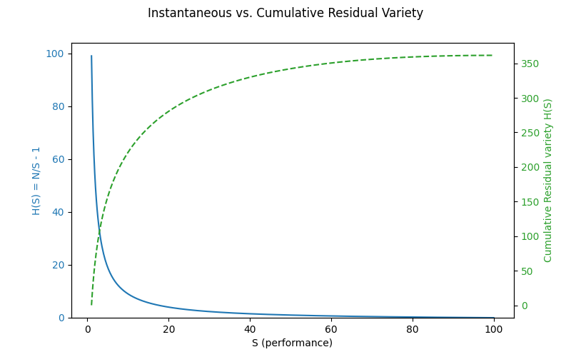
**Fig.2 Total Knowledge-Effort Curve** Here we see the cumulative residual variety as a function of performance level.

Blue curve: instantaneous 𝐻(𝑆)=𝑁/𝑆−1H(S)=N/S−1 (residual variety ratio).

Green dashed curve: cumulative residual variety C(S) as we accumulate uncertainty over growing performance level S.

Each point on the curve says “At performance level S, there are *H(S)* bits of uncertainty to be eliminated for perfect regulation.” We can see how H(S) declines hyperbolically, while C(S) rises concavely.

How to cite:

Bakardzhiev D.V. (2025) Knowledge Discovery Efficiency (KEDE) and Ashby's Law https://docs.kedehub.io/knowledge-centric-research/kede-ashbys-law.html

Works Cited

1. Shannon, C. E. (1948). A Mathematical Theory of Communication. Bell System Technical Journal. 1948;27(3):379-423. doi:10.1002/j.1538-7305.1948.tb01338.x

2. Ashby, W.R. (1956). An Introduction to Cybernetics; Chapman & Hall,

3. Ashby, W. R. (2011). Variety, Constraint, And The Law Of Requisite Variety. 13, 18.

4. MacKay, D. M. (1950). Quanta! aspects of scientific information. Philosophical Magazine; 41, 289-311;

5. Cover, T. M. & Thomas, J. A. (2006). Elements of Information Theory, 2nd ed., Wiley. §5.2–5.5 (Kraft, entropy bound, source coding bracket), §5.7 (Huffman codes and twenty questions), §2.8 (data-processing inequality).

6. Wheeler, J. A. (1990). Information, physics, quantum: The search for links. In W. H. Zurek (Ed.), Complexity, entropy, and the physics of information (Vol. 8, pp. 3'-28). Taylor & Francis.

7. Yaneer Bar-Yam.(2004) Multiscale variety in complex systems. Complexity, 9(4):37{45,

8. Ashby, W.R. (1991). Requisite Variety and Its Implications for the Control of Complex Systems. In: Facets of Systems Science. International Federation for Systems Research International Series on Systems Science and Engineering, vol 7. Springer, Boston, MA. https://doi.org/10.1007/978-1-4899-0718-9_28

9. Shannon, C. E. Communication theory of secrecy systems. Bell System technical Journal, 28, 656-715, 1949

10. Kubatko J, Oliver D, Pelton K, et al. A starting point for analyzing basketball statistics. J Quant Anal Sports 2007; 3: 1'-22.

11. Sports Reference LLC. "NBA League Averages." Basketball-Reference.com - Basketball Statistics and History. https://www.basketball-reference.com/leagues/NBA_stats_totals.html.

12. Bucks post highest single-game field-goal percentage by any team in 21st century https://sports.yahoo.com/article/bucks-post-highest-single-game-040313061.html

13. https://www.statmuse.com/nba/ask/most-field-goals-made-record-in-a-game-nba-player

14. Lewis, G. J., & Stewart, N. (2003). The measurement of environmental performance: an application of Ashby's law. Systems Research and Behavioral Science, 20(1), 31'-52. https://doi.org/10.1002/sres.524

15. Norman, J., & Bar-Yam, Y. (2018). Special Operations Forces: A Global Immune System? In Springer Unifying Themes in Complex Systems IX (pp. 486'-498). Springer International Publishing. https://doi.org/10.1007/978-3-319-96661-8_50

16. Norman, J., & Bar-Yam, Y. (2019). Special Operations Forces as a Global Immune System. In Springer Evolution, Development and Complexity (pp. 367'-379). Springer International Publishing. https://doi.org/10.1007/978-3-030-00075-2_16

17. O'Grady, W., Morlidge, S., & Rouse, P. (2014). Management Control Systems: A Variety Engineering Perspective. SSRN Electronic Journal. https://doi.org/10.2139/ssrn.2351099

18. Love, T., & Cooper, T. (2007). Digital Eco-systems Pre-Design: Variety Analyses, System Viability and Tacit System Control Mechanisms. 2007 Inaugural IEEE-IES Digital EcoSystems and Technologies Conference, 452'-457. https://doi.org/10.1109/dest.2007.372013

19. Love, T., & Cooper, T. (2007). Complex built‐environment design: four extensions to Ashby. Kybernetes, 36(9/10), 1422'-1435. https://doi.org/10.1108/03684920710827391

20. Bushey, D. B., & Nissen, M. E. (1999). A Systematic Approach to Prioritizing Weapon System Requirements and Military Operations Through Requisite Variety. Defense Technical Information Center. https://doi.org/10.21236/ada371943

21. Jones, H. P. (2018). Evolutionary stakeholder discovery: requisite system sampling for co-creation.

22. Grimm, D. A. P., Gorman, J. C., Robinson, E., & Winner, J. (2022). Measuring Adaptive Team Coordination in an Enroute Care Training Scenario. Proceedings of the Human Factors and Ergonomics Society Annual Meeting, 66(1), 50'-54. https://doi.org/10.1177/1071181322661074

23. Becker Bertoni, V., Abreu Saurin, T., & Sanson Fogliatto, F. (2022). Law of requisite variety in practice: Assessing the match between risk and actors' contribution to resilient performance. Safety Science, 155, 105895. https://doi.org/10.1016/j.ssci.2022.105895

24. Tworek, K., Walecka-Jankowska, K., & Zgrzywa-Ziemak, A. (2019). Towards organisational simplexity — a simple structure in a complex environment. Engineering Management in Production and Services, 11(4), 43'-53. https://doi.org/10.2478/emj-2019-0032

25. Chester, M. V., & Allenby, B. (2022). Infrastructure autopoiesis: requisite variety to engage complexity. Environmental Research: Infrastructure and Sustainability, 2(1), 012001. https://doi.org/10.1088/2634-4505/ac4b48

26. van der Hoek, M., Beerkens, M., & Groeneveld, S. (2021). Matching leadership to circumstances? A vignette study of leadership behavior adaptation in an ambiguous context. International Public Management Journal, 24(3), 394'-417. https://doi.org/10.1080/10967494.2021.1887017

27. Ulrik, S., & Isabella, A. (2023). Variety versus speed: how variety in competence within teams may affect performance in a dynamic decision-making task.

28. Bakardzhiev, D., Vitanov, N.K. (2025). KEDE (KnowledgE Discovery Efficiency): A Measure for Quantification of the Productivity of Knowledge Workers. In: Georgiev, I., Kostadinov, H., Lilkova, E. (eds) Advanced Computing in Industrial Mathematics. BGSIAM 2022. Studies in Computational Intelligence, vol 641. Springer, Cham. https://doi.org/10.1007/978-3-031-76786-9_3

29. Heylighen, F., & Joslyn, C. (2001). Cybernetics and Second Order Cybernetics. In R. A. Meyers (Ed.), Encyclopedia of Physical Science and Technology, Eighteen-Volume Set, Third Edition (pp. 155-170). Academia Press. http://pespmc1.vub.ac.be/Papers/Cybernetics-EPST.pdf

30. Schwaninger, M., & Ott, S. (2024). What is variety engineering and why do we need it? Systems Research and Behavioral Science, 41(2), 235'-246. https://doi.org/10.1002/sres.2964

31. AULIN‐AHMAVAARA, A.Y. (1979), "THE LAW OF REQUISITE HIERARCHY", Kybernetes, Vol. 8 No. 4, pp. 259-266. https://doi.org/10.1108/eb005528

32. Wu, T., Dufford, A. J., Mackie, M. A., Egan, L. J., & Fan, J. (2016). The Capacity of Cognitive Control Estimated from a Perceptual Decision Making Task. Scientific Reports, 6, 34025.

33. Abuhamdeh S (2020) Investigating the “Flow” Experience: Key Conceptual and OperationalIssues. Front. Psychol. 11:158.doi: 10.3389/fpsyg.2020.00158

34. Automatic Screw Tightening Machine and Its Hidden Features

35. Keating, C. B., Katina, P. F., Jaradat, R., Bradley, J. M., & Hodge, R. (2019). Framework for improving complex system performance. INCOSE International Symposium, 29(1), 1218-1232. https://doi.org/10.1002/j.2334-5837.2019.00664.x

36. S. Engell (1985). An information-theoretical approach to regulation.

37. K. Kijima, Y. Takahara, B. Nakano (1986). ALGEBRAIC FORMULATION OF RELATIONSHIP BETWEEN A GOAL SEEKING SYSTEM AND ITS ENVIRONMENT.

38. W. Kickert, J. Bertrand, J. Praagman (1978). Some Comments on Cybernetics and Control. IEEE Transactions on Systems, Man and Cybernetics.

39. S. Engell (1985). Information-theoretical bounds for regulation accuracy. IEEE Conference on Decision and Control.

40. Hui Zhang, Youxian Sun (2003). Bode integrals and laws of variety in linear control systems. Proceedings of the 2003 American Control Conference, 2003.

41. R. Conant (1969). The Information Transfer Required in Regulatory Processes. IEEE Transactions on Systems Science and Cybernetics.

42. S. Engell (1987). Analysis of Regulation Problems based on Real-Time Rate-Distortion Theory. American Control Conference.

43. Hui Zhang, Youxian Sun (2003). Information theoretic limit and bound of disturbance rejection in LTI systems: Shannon entropy and H/sub /spl infin// entropy. SMC'03 Conference Proceedings. 2003 IEEE International Conference on Systems, Man and Cybernetics. Conference Theme - System Security and Assurance (Cat. No.03CH37483).

44. N. C. Martins, M. Dahleh (2008). Feedback Control in the Presence of Noisy Channels: “Bode-Like” Fundamental Limitations of Performance. IEEE Transactions on Automatic Control.

45. Hui Zhang, Youxian Sun (2003). H/sub /spl infin// entropy and the law of requisite variety. 42nd IEEE International Conference on Decision and Control (IEEE Cat. No.03CH37475).

46. Tsuji, M., Crookshank, M., Olsen, M., Schemitsch, E. H., & Zdero, R. (2013). The biomechanical effect of artificial and human bone density on stopping and stripping torque during screw insertion. Journal of the mechanical behavior of biomedical materials, 22, 146'-156. https://doi.org/10.1016/j.jmbbm.2013.03.006

47. Akizuki, K., & Ohashi, Y. (2015). Measurement of functional task difficulty during motor learning: What level of difficulty corresponds to the optimal challenge point?. Human movement science, 43, 107'-117. https://doi.org/10.1016/j.humov.2015.07.007

48. Bootsma, J. M., Hortobágyi, T., Rothwell, J. C., & Caljouw, S. R. (2018). The Role of Task Difficulty in Learning a Visuomotor Skill. Medicine and science in sports and exercise, 50(9), 1842'-1849. https://doi.org/10.1249/MSS.0000000000001635

49. Akizuki, K., & Ohashi, Y. (2013). Changes in practice schedule and functional task difficulty: a study using the probe reaction time technique. Journal of physical therapy science, 25(7), 827'-831. https://doi.org/10.1589/jpts.25.827

50. Goldhammer, F.; Naumann, J.; Stelter, A.; Tóth, K.; Rölke, H.; Klieme, E.: The time on task effect in reading and problem solving is moderated by task difficulty and skill. Insights from a computer-based large-scale assessment - In: The Journal of educational psychology 106 (2014) 3, S. 608-626 - URN: urn:nbn:de:0111-pedocs-179679 - DOI: 10.25656/01:17967; 10.1037/a0034716

51. Boothroyd, G., and P. Dewhurst, "DESIGN FOR ASSEMBLY", Dept. of Mechanical Engineering, University of Massachusetts, Amherst, Massachusetts, 1983.

52. Jahin, A., Zidan, A. H., Bao, Y., Liang, S., Liu, T., & Zhang, W. (2025). Unveiling the mathematical reasoning in deepseek models: A comparative study of large language models. arXiv preprint arXiv:2503.10573.

53. FrontierMath: A Benchmark for Evaluating Advanced Mathematical Reasoning in AI

54. Francis Heylighen, Cybernetic Principles of Aging and Rejuvenation: The Buffering- Challenging Strategy for Life Extension, Current Aging Science; Volume 7, Issue 1, Year 2014, . DOI: 10.2174/1874609807666140521095925

55. Ostry, D. J. (1980). Execution-time movement control. In G. E. Stelmach & J. Requin (Eds.), Tutorials in motor behavior (pp. 457-468). Amsterdam: North-Holland.

56. Siegenfeld, A. F., & Bar-Yam, Y. (2025). A Formal Definition of Scale-Dependent Complexity and the Multi-Scale Law of Requisite Variety. Entropy, 27(8), 835. https://doi.org/10.3390/e27080835

57. Umpleby, S. A. (2009). Ross Ashby's general theory of adaptive systems. International Journal of General Systems, 38(2), 231–238. https://doi.org/10.1080/03081070802601509

58. Zheng, J., & Meister, M. (2024). The unbearable slowness of being: Why do we live at 10 bits/s?. Neuron.

59. Ohlsson, S. (1992). The Learning Curve for Writing Books: Evidence from Professor Asimov. Psychological Science, 3(6), 380-382.

60. L. B.S. Raccoon. 1996. A learning curve primer for software engineers. SIGSOFT Softw. Eng. Notes 21, 1 (Jan 1 1996), 77–86. https://doi.org/10.1145/381790.381805

61. Deweese, M. R., & Meister, M. (1999). How to measure the information gained from one symbol. Network: Computation in Neural Systems, 10(4), 325–340. https://doi.org/10.1088/0954-898X_10_4_303

62. Gallager, R. G. (1978). Variations on a theme by Huffman. IEEE Trans. Inform. Theory 24(6), 668–674. (Redundancy bound p_{\max} + 0.086.)

63. MacKay, D. J. C. (2003). Information Theory, Inference, and Learning Algorithms, CUP, ch. 5 (Ex. 5.24, 5.28).

64. McMillan, B. (1956). Two inequalities implied by unique decipherability. IRE Trans. Inform. Theory 2(4), 115–116. (Optional; Cover & Thomas suffices.)

65. Azuma, K. (1967). Weighted sums of certain dependent random variables. Tôhoku Math. J. 19, 357–367; Hoeffding, W. (1963). Probability inequalities for sums of bounded random variables. JASA 58, 13–30. (For Theorem 2(iv).)

Getting started

Frequently Asked Questions

About KEDE and KEDEHub

KEDEHub Features

All we need to analyze the efficiency of your organization

Knowledge-Centric Metrics

The complete set of concepts, terms and theories

Need help?

KEDEHub Documentation

Knowledge Discovery Efficiency (KEDE) and Ashby's Law of Requisite Variety

Related Articles

Abstract

Introduction

Core challenges in applying Ashby's Law to real systems

Solution

The Law of Requisite Variety

Set-based formulation

Requisite variety

Outcome map induced by a response rule at time t

Goal revision with fixed table and time-indexed acceptable outcomes

Revision of acceptability: deletion, addition, and substitution within the acceptable outcome-set

Strict substitution

Behavioral rework

Information-Theoretic Formulation

Random variables over the set-based regulatory geometry

Entropy, variety, and the outcome-to-essential-variable map

Probabilistic success and support-level success

Allowed residual variety

Response-equivalence and regulatory ignorance

Regulator's learned law of action

Knowledge To Be Discovered

Knowledge To Be Discovered and effective regulatory knowledge

Ashby-style residual-variety bounds

Point regulation

Knowledge Discovery Process

Set-based Formulation of Staged Selection

Rule regulation

Episodes and Closures

Action-unit protocols

Count-Variety Selection

Information-Theoretic Formulation of Staged Selection

What the Information-Theoretic Model Adds

Notation and Modeling Assumptions

Staged Action Units and Realized Signals

Expected Staged Reduction of Knowledge To Be Discovered

Realized Conditioning Path Inside One Episode

Form of the realized stage-information functional

Realized stage information

Why specific surprise is not the stage-flow measure

Terminal realized Knowledge To Be Discovered

Fixed-model scope of the specific-information result

Bridge to the Set-Based Candidate Trace

Bridge Lemma: epistemic support and terminal real KTD

Action Units, Signals, and Response-Class Commitment

Success, Closure, and Policy-Level Success

Summary

Learning (across episodes in a window)

Comparable episodes

Learning as stored transformation

From staged discovery to stored learning

Across-episode comparison of stored coupling

Learning axiom

Strong learning: posterior becomes prior

Learning, goal revision, and behavioral revision

Knowledge Discovery Accounting

Operational ledger

Closure events

Window

Gross counted closures

Historically realized outcome-set

Continuously surviving counted closures through the window

Invalidation load

Interpretation

Operational ledger for goal-model revision

Authoritative and believed acceptability

Provisional closure events

Provisional closure history

Gross provisional closures

Net surviving closures

Goal-model invalidation load

Ledger identity

Model-revision events

Corrective replacement

Relation to the criterion-revision ledger

Interpretation

Operational counting of action units as Effective non-net-progress load

Knowledge ledger

Closure-indexed knowledge ledger

KTD states at closure boundaries