KEDE Learning Curve

Abstract

The concept of a learning curve is not just a theoretical construct but a practical tool for managing software development. The learning curve model helps monitor various aspects of company performance and identify areas that need improvement. It provides insights into employee training and capability.

This article delves into the intricacies of the learning curve in software development, a domain where continuous learning and adaptation are not just beneficial but essential for success. The learning curve here is not merely about the time and effort required to grasp new technologies, programming languages, frameworks, and methodologies; it's about quantifying and optimizing the process of knowledge discovery and application. By adopting a Knowledge-Centric approach, we aim to measure this effort in tangible units - bits of information - offering a clear perspective on how knowledge fuels the engine of software development.

As we explore the various facets of learning curves, we will discuss their types, implications in different project environments, and the methods to compare them effectively across diverse projects. This exploration is not just an academic exercise but a practical guide to understanding how software development teams can enhance their productivity by efficiently managing the learning process.

The Learning Curve in Software Development

The learning curve in software development encapsulates the time and effort required to learn new technologies, programming languages, frameworks, and methodologies. It assigns an improvement value to gauge the efficiency rate as task performers learn and become more proficient[3]. Adopting a Knowledge-Centric approach, we measure this effort in bits of information, treating knowledge as the fuel that drives the software development engine.

Prior knowledge significantly influences learning efficiency, as it provides a foundation upon which new information is built[4]. Additionally, prior knowledge of different domains can jointly support the recall of arguments[5].

This interpretation aligns with the economic understanding of learning curves, where the focus is on the relationship between the amount of learning (or experience) and productivity. It underscores the importance of recognizing and managing these learning phases for the successful execution of software development projects.

Visualizing a learning curve

The learning curve can be visualized by tracking the cumulative amount of knowledge discovered over time. For instance, consider a diagram illustrating the knowledge growth in bits for a specific project.

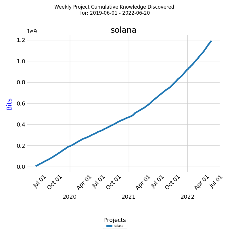
Over the given period, the total knowledge discovered accumulated to 1.2*109 bits or 1.2 terabits (Tbits). The blue line marks the cumulative knowledge growth, reflecting the team's advancement in the project.

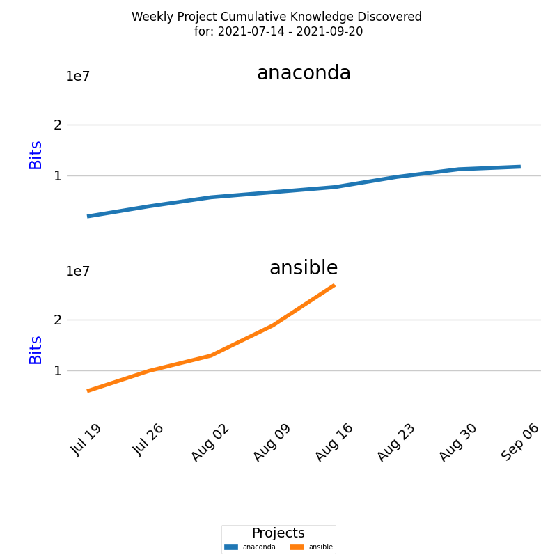
To facilitate meaningful comparisons across software development projects with varying scales of knowledge acquisition, normalization of data is essential. Direct comparisons based on raw knowledge values, measured in bits, can be misleading due to differences in project scale, as visible on the diagram below.

Learning rate measured in bits of information discovered per unit of time, is a critical aspect of this curve. The higher the learning rate, the faster the knowledge discovery process.

In the context of learning curves, especially from an economic perspective, a high learning rate typically corresponds to a period where there is a lot of new learning taking place, such as when new technologies or methodologies are being introduced. This is because the learning rate is a measure of the speed at which new knowledge is acquired.

High Learning Rate: When a team is faced with new technologies or methodologies, they have a lot to learn. This period of intense learning is characterized by a high learning rate. The team is rapidly acquiring new knowledge, even though their immediate productivity might be lower due to the time and effort required to assimilate this new information. Although their immediate productivity might be lower due to the time and effort required to assimilate this new information, this phase is crucial for long-term capability building.
Low Learning Rate: Conversely, when the team is working on routine, well-understood tasks, the learning rate is lower because there is less new knowledge to acquire. The team is applying existing knowledge, which typically correlates with higher productivity. This phase is essential for achieving immediate project goals and deliverables.

Understanding these varying learning rates is vital for effective project planning and management. For instance, a project in its initial stages, involving new technologies, might require additional time and resources to accommodate the higher learning rate. Conversely, projects in later stages, focusing on application and refinement, might progress more rapidly due to the lower learning rate.

Let's consider a hypothetical scenario: a software development team working on a cutting-edge project. Initially, they invest significant time in learning and experimenting with new technologies (high learning rate), which might slow down initial progress. However, as they become more proficient, their focus shifts to applying this knowledge to develop innovative solutions, leading to increased productivity (low learning rate).

We employ the cumulative growth rate (CR) of knowledge discovered as a key metric for measuring normalized growth. CR effectively normalizes growth by taking into account variations in project sizes, durations, and initial knowledge levels. This approach transforms CR into a relative measure, enabling fair and equitable comparisons across diverse projects. The methodology for calculating CR is detailed in the Appendix.

CR's ability to adjust for different project lengths and initial knowledge states offers a more nuanced perspective on growth than mere absolute knowledge figures. The accompanying diagram illustrates this point by comparing two distinct projects. Despite their differing total knowledge growth, CR reveals a more comparable rate of knowledge acquisition when normalized.

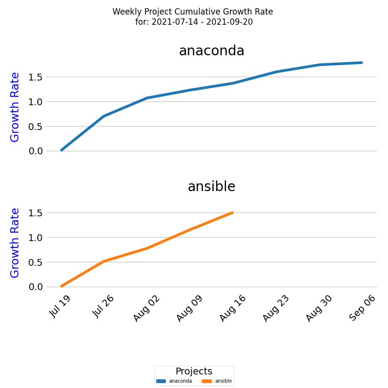
In the diagram, the x-axis represents the timeline (in weeks), while the y-axis denotes the cumulative growth rate. The lines trace the exponential cumulative growth rate for each project over the specified period. It's crucial to recognize that the actual cumulative growth rate of a project is influenced by a unique combination of factors that drive the knowledge discovery process.

This comparative visualization underscores the utility of CR in providing a balanced view of project performance, especially in scenarios where project scopes or complexities vary significantly. However, it's important to consider that while CR offers valuable insights, it may not capture all qualitative aspects of knowledge growth, and external factors might also impact the learning curve.

Types of Learning Curve

In the field of software development, understanding the nuances of learning curves is crucial for managing projects effectively. A learning curve represents the rate of knowledge discovery and application within a project environment. This concept is particularly relevant in software development, where knowledge serves as the fuel driving the creation and refinement of technology solutions.

The efficiency of knowledge discovery and application plays a pivotal role in determining the productivity of a software development team. Teams that excel in applying existing knowledge efficiently are often more productive, as they can deliver outcomes without the constant need for assimilating new information. This efficiency is reflected in the learning curve, which illustrates the rate at which a team acquires and applies knowledge over time.

If software developers don't have the knowledge needed they have to discover it. The knowledge they have to discover is the total of what they don't know they don't know and what they know they don't know. Prior knowledge, being readily available, is the easiest and fastest to apply, leading to efficient knowledge discovery. Conversely, when substantial knowledge is missing, discovery becomes less efficient. Optimal productivity is achieved when minimal new knowledge discovery is required for outcomes.

There are three different types of learning curves. We present them visually on the below diagram.

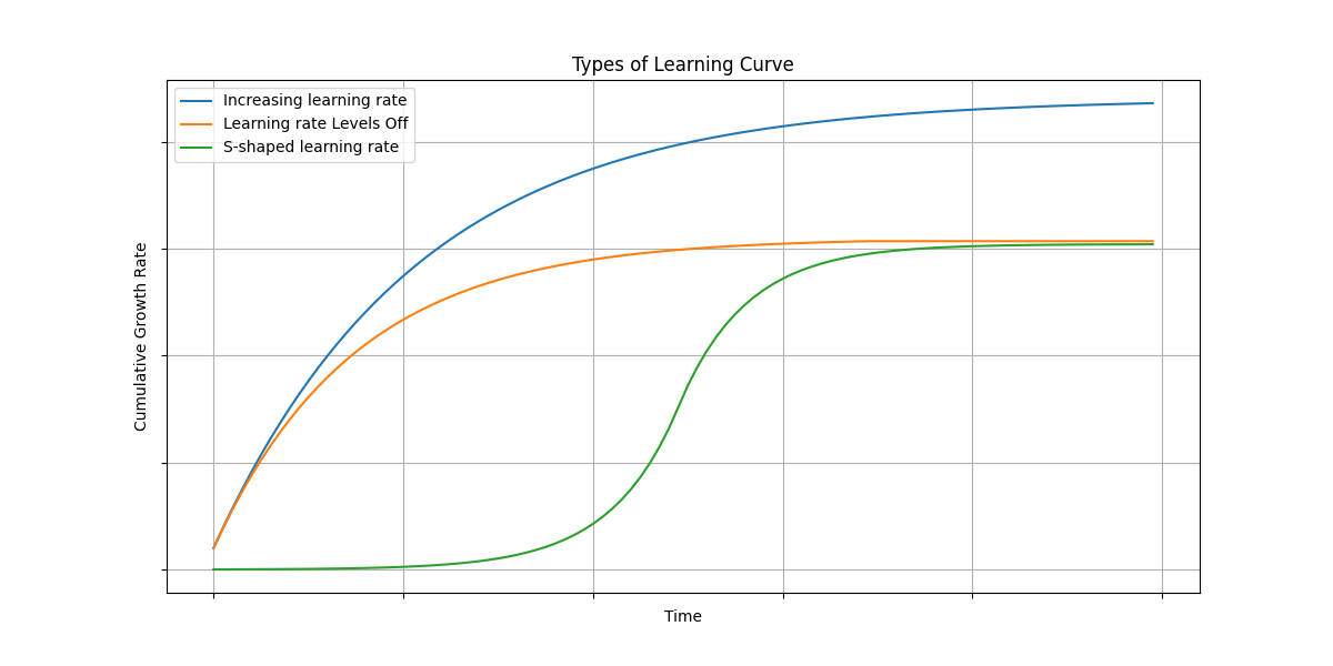
Each type provides insights into the dynamics of knowledge discovery and application, reflecting different project environments and stages of development.

Here's a short description for each of the three learning curve types measured using the Cumulative Growth Rate (CR) of knowledge discovered, along with insights into what each type might reflect about a project environment:

Increasing learning rate:
- Description: This curve shows a consistent increase in the learning rate over time, indicating that the rate of knowledge discovery is steadily growing.
- Project Environment Implication: This scenario might reflect a highly innovative environment where continuous experimenting and discovery are encouraged, and new challenges or technologies are frequently introduced. It might also indicate challenges or obstacles that are hindering learning and growth, such as ineffective knowledge sharing and collaboration, resource constraints, loss of key personnel, or a shift in project goals. For knowing the real cause we need to look inside the organization. Here is a case study of a blockchain company.
- Example scenario in real-world projects: A startup working on an innovative blockchain project. In the early stages, the team has a basic understanding of blockchain but needs to rapidly adapt to emerging technologies and methodologies. As the project progresses, they continuously encounter new challenges requiring novel solutions, leading to a consistently increasing learning rate.
Learning rate Levels Off:
- Description: The learning rate initially increases but then reaches a plateau, indicating that the rate of new knowledge discovery slows down and stabilizes.
- Project Environment Implication: This pattern is often seen in projects with a clear development, growth, and support phase, such as technology implementation projects. The initial fast growth represents a phase of rapid learning and low productivity, where there is accumulation of new knowledge. The slowdown indicates a phase of working on already well understood tasks, probably with high productivity. Finally, the project matures, and the rate of encountering new knowledge stabilizes. The leveling off suggests that while new knowledge is still being gained, the rate of learning has decreased, possibly due to the team becoming more experienced and encountering fewer unknowns. This pattern is typical of a mature project environment where the team has acquired substantial knowledge and established stable processes. This could also reflect a shift in focus away from exploration and towards optimization or routine work as the project goes into support mode.
- Example scenario in real-world projects: A software development team working on a long-term enterprise resource planning (ERP) implementation. Initially, there's a steep learning curve as the team familiarizes itself with the client's unique requirements and how they could be implemented with the specific ERP software. Over time, as they gain expertise, the learning rate stabilizes, and the team becomes more efficient in applying their knowledge.
S-shaped learning rate:
- Description: The learning rate curve starts with a slow knowledge growth, accelerates to a peak rate of knowledge discovery, and then slows down again, forming an S-shape.
- Project Environment Implication: This pattern is also often seen in projects that go through distinct phases. The initial slow growth of knowledge discovered represents working on routine, well understood tasks, leading to higher productivity. That could probably be done to make a good impression of high productivity. The acceleration indicates a phase of rapid learning and low productivity. As the curve progresses and the learning rate increases, this could indicate a phase where the team is encountering the real challenges of the work to be done, requiring more learning and potentially experiencing a temporary dip in productivity. Finally, the slowdown occurs as the project matures, and the rate of encountering new knowledge decreases. From a project management perspective, this is a wrong way, because they tried to deny the reality of software development, which is a constant acquisition and application of new knowledge.
- Example scenario in real-world projects: A software development team is tasked with creating a new mobile application. Initially, they focus on basic functionality using familiar technologies, leading to a low learning rate and high productivity. However, as they start integrating advanced features like machine learning for personalized user experiences, the learning rate accelerates and productivity lowres. Eventually, as the major challenges are addressed and the team becomes proficient, the learning rate slows down and productivity improves again.

Each of these learning curve types not only reflects the rate of knowledge acquisition but also provides insights into the project's complexity, the team's adaptability, and the overall project lifecycle. By analyzing the learning rate, project managers and teams can better understand their learning environment, identify areas for improvement, and make informed decisions about resource allocation, training, and process adjustments.

Comparing learning curves

To effectively compare projects of varying durations, we need a method that can handle empirical data from each curve without requiring the analytical function of the curves. Given that we're dealing with time series data, alignment and stretching of the data points are crucial considerations.

We have chosen Dynamic Time Warping (DTW) as our primary method for measuring the similarity between two time series. DTW measures the similarity between two time series by minimizing the distance between their points, allowing for non-linear time alignment. A smaller DTW distance between two curves indicates a higher degree of similarity. This method is particularly beneficial when the curves have similar shapes but are misaligned in time or exhibit different progression speeds.

For clustering the curves, we opt for Hierarchical Clustering. This algorithm is well-suited for our purpose as it does not presuppose any specific shape for the clusters. It also provides the flexibility to visualize the hierarchy of clusters, aiding in the selection of an appropriate number of clusters. However, it's important to note that Hierarchical Clustering may not always be the optimal method, especially when dealing with a small number of curves, or when the curves are not significantly distinct in their distances.

Utilizing these methods, we can compare the knowledge discovery processes across different projects. The accompanying diagram illustrates six project curves:

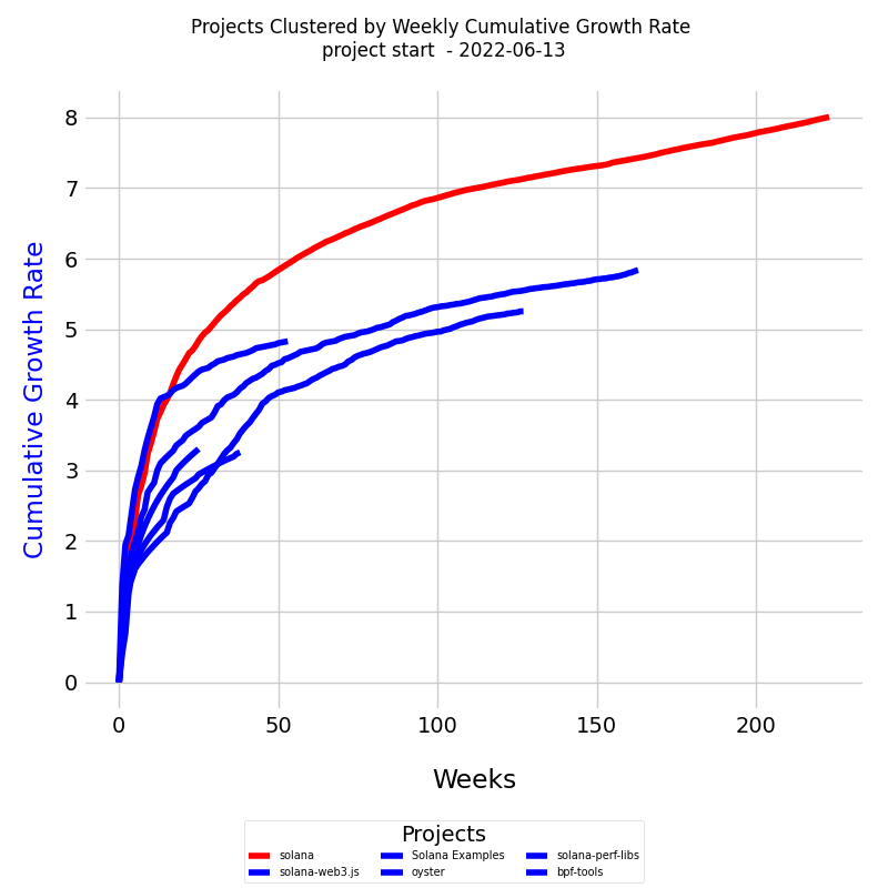
In this diagram, we have plotted six CR_T curves, considering their varying lengths in time units. The curves are color-coded based on the clusters derived from DTW distances.

Conclusion

The exploration of learning curves in software development reveals a complex yet fascinating aspect of how knowledge is acquired, applied, and managed in project environments. Our journey through the different types of learning curves - increasing, leveling off, decreasing, and S-shaped - provides valuable insights into the dynamics of knowledge discovery and application. These insights are crucial for project managers and team members to understand their learning environment, identify areas for improvement, and make informed decisions about resource allocation, training, and process adjustments.

The application of Dynamic Time Warping (DTW) and Hierarchical Clustering to compare learning curves across projects further enhances our understanding of these dynamics. These methods allow us to measure the similarity between learning curves and group them effectively, even when they vary in length and progression speed. The resulting analysis not only aids in comparing the knowledge discovery process across different projects but also in drawing meaningful conclusions about the efficiency and effectiveness of learning in software development.

In conclusion, the learning curve in software development is a powerful tool for gauging and improving the efficiency of knowledge discovery and application. By understanding and leveraging the nuances of learning curves, software development teams can optimize their learning processes, leading to increased productivity and success in their projects.

Appendix

Exponential growth

The concept of cumulative growth rate is widely used in finance to measure the performance of investments or financial assets over time. For example, an investor might calculate the cumulative growth rate of a stock or a mutual fund over a certain period to determine the overall return on their investment. The cumulative growth rate can also be used to compare the performance of different investments over the same time period. Moreover, cumulative growth rate is also useful in analyzing economic growth or population growth over time.

In finance, compound returns cause exponential growth. The power of compounding is one of the most powerful forces in finance. This concept allows investors to create large sums with little initial capital. Savings accounts that carry a compound interest rate are common examples of exponential growth.

To calculate the cumulative growth rate we'll be using an exponential growth model. Exponential growth models describe a quantity that grows at a rate proportional to its current value. The general form of an exponential growth model is:

$y (t) = y (0) e^{k t}$

where y(t) is the value of the quantity at time t, y(0) is the initial value, k is the growth rate, and e is the base of the natural logarithm.

There are two cases - when the exponential growth rate over the interval from t=0 to t=T-1. is a constant and when it changes over time.

Constant exponential growth rate

To calculate the exponential growth rate of knowledge discovered Q, we can use the following general formula:

$R = \frac{d Q (t)}{Q (t)}$

The general formula calculates the exponential growth rate based on the ratio of the rate of change of knowledge discovered dQ/dt to the knowledge discovered Q at each time point.

If we know the initial knowledge discovered Q(0) and the exponential growth rate, we can calculate the knowledge discovered at a later time, such as Q(T), assuming the exponential growth rate remains constant over the given time interval.

To find the value of Q(T), we need to integrate this equation. For this purpose, we can use the following steps:

Rearrange the equation: dQ(t) / Q(t) = R
Integrate both sides with respect to time (t): ∫(dQ(t) / Q(t)) dt = ∫(R) dt
The integral of the left-hand side is the natural logarithm of Q(t): ln(Q(t)) = R * t + C
Solve for Q(t): Q(t) = e^(R * t + C)
Now, you can use the initial condition Q(0) to find the constant C:
Q(0) = e^(R * 0 + C) = e^C

C = ln(Q(0))

Finally, you can find Q(T) using the formula:

$Q_{T} = e^{R T + \ln (Q_{0})} = Q_{0} e^{R T}$

This calculation assumes a constant exponential growth rate over the interval from t=0 to t=T-1.

Cumulative growth rate of knowledge discovered

When the exponential growth rate changes over time, we would need to know the function describing its change or have a time-series of exponential growth rates to calculate knowledge discovered Q(T).

In finance, the natural logarithm (ln) of the ratio between the future value and the current value of a financial asset is often used to calculate the exponential growth rate. This is referred to as the logarithmic or log return and measures the rate of exponential growth during a specific time period.

$R (t) = \ln (\frac{\sum_{i = 1}^{t + 1} Q (i)}{\sum_{i = 1}^{t} Q (i)})$

The log return R_t at a specific time step t represents the logarithm of the ratio of the sum of the knowledge acquired up to time t+1 to the sum of the knowledge acquired up to time t. The log return measures the relative growth in knowledge between two consecutive time steps, with higher values indicating faster growth.

The log return for a time period is the sum of the log returns of partitions of the time period. For example the log return for a year is the sum of the log returns of the days within the year. We will cal this cumulative growth rate because it is more proper for the context of knowledge management in projects.

The cumulative growth rate CR_T over the duration of the project up to time T is calculated using the formula:

$C R_{T} = \sum_{t = 0}^{T - 1} R (t)$

CR_T is the sum of the log returns R_t at each time step t from the beginning of the project (t=0) to the end of the project (t=T-1). CR_T represents the overall rate of knowledge growth in the project. The cumulative growth rate CR_T represents the proportionality constant for the growth of knowledge discovered H_T over time.

To calculate the total knowledge discovered Q_T at a given time T, we use the formula:

$Q_{T} = Q_{0} e^{C R_{T}}$

Here, Q₀ represents the initial knowledge at the beginning of the project, and e^CR_T represents the exponential growth factor driven by the growth rate CR_T. The total knowledge discovered at time T is the product of the initial knowledge and the exponential growth factor.

Together, these three formulas provide a framework for quantifying and tracking the growth of knowledge in a project over time. By calculating the log returns R_t and cumulative growth rate CR_T, we can gain insights into the dynamics of knowledge discovery and make comparisons between different projects or strategies.

Using the cumulative growth rate (CR) instead of the time-series of knowledge discovered when comparing projects offers several advantages:

Normalization: CR is derived from the og returns (R), which inherently normalize the growth rates and allow for a more meaningful comparison across projects with varying magnitudes of knowledge discovered. Comparing raw Q values may be misleading, as differences in scale can distort the true relative performance between projects.
Relative performance: CR captures the overall rate of knowledge discovery throughout the project duration, making it possible to evaluate the relative performance of different projects, strategies, teams, or methodologies. By comparing the cumulative growth rates, you can determine which project experienced a higher overall rate of knowledge growth. In contrast, comparing Q values directly may not provide the same level of insight into relative performance, as it focuses on the absolute amount of knowledge discovered rather than the rate of growth.
Stability: CR is generally more stable and less susceptible to fluctuations due to random or transient events. By summing up all log returns (R) over the project duration, CR smooths out short-term variations and captures the overall trend of knowledge growth. This provides a more reliable basis for comparison between projects, as it minimizes the impact of noise or isolated events. Comparing Q values directly may be more sensitive to such fluctuations, making it harder to discern underlying trends.
Simplicity: CR provides a single, summary metric that encapsulates the overall knowledge growth across the entire project lifecycle. This simplifies the comparison process by reducing the complexity of the data and allowing for a more straightforward interpretation of results. Comparing time-series of Q values requires evaluating a multitude of data points, making it more challenging to draw meaningful conclusions.

Total exponential growth rate for N developers

Calculating the exponential growth rate R_t for each of the N developers and then summing it will not be an accurate representation of the total exponential growth rate. The reason for this is that exponential growth rates are not additive.

The correct approach to calculate the total exponential growth rate at each time point t for N developers, we first need to calculate the sum of knowledge discovered Q for all developers at each time point. Then, we will use the given formula:

$R (t) = \ln (\frac{\sum_{i = 1}^{t + 1} Q (i)}{\sum_{i = 1}^{t} Q (i)})$

to calculate the exponential growth rate R_t. By doing this, we take into account the combined effect of all developers on the system's knowledge growth.

Here's a step-by-step process:

Calculate the sum of knowledge discovered Q for all developers at each time point.
Calculate the exponential growth rate R_t.

Clustering algorithms

When dealing with curves that follow a logarithmic pattern, the choice of clustering algorithm can still be influenced by various factors such as the number of clusters, the noise in the data, and other domain-specific considerations.

Here are some popular clustering algorithms that might be suitable for your task

K-Means Clustering: K-Means is a popular and easy-to-implement clustering algorithm. Although it assumes that clusters are convex and isotropic (i.e., the same in all directions), it can still be effective in many real-world situations. If you know the approximate number of clusters, you could try K-Means.
Hierarchical Clustering: This algorithm is a good choice for clustering curves. It does not assume any particular shape for the clusters, and it allows you to visualize the hierarchy of clusters to choose an appropriate number.
Hierarchical clustering may not be the best method for separating a small number of curves, especially when the number of clusters is equal to the number of curves or when the distances between the curves are not significantly different.
Gaussian Mixture Model (GMM): A Gaussian Mixture Model is a probabilistic model that assumes that the data is generated from several Gaussian distributions. If the data fits this assumption, GMM might be a good choice.
DBSCAN: DBSCAN does not require the number of clusters to be specified and can find clusters of arbitrary shape, making it a good option for data that doesn't meet the assumptions of K-Means.

As with many machine learning tasks, the "best" algorithm may depend heavily on the specifics of your data and what exactly you want to achieve. Experimenting with different algorithms and validating the results using appropriate evaluation metrics will likely be necessary to find the optimal solution for your particular problem.

If the curves are logarithmic, using a distance metric that takes into account the underlying pattern may be more important than the choice of the clustering algorithm itself.

Heaps' Law

The Heaps law, introduced by Heaps in 1978 [1], is an empirical law that describes the number of different elements D(N) occurring in a sequence of length N when N is large, with the following rule:

$D (N) = N^{β}, β \in (0, 1)$

(1)

The sub-linear growth is a result of the exponent β being less than 1.

Heaps' law was first introduced to describe the number of distinct words in a document as a function of the document's length. That is it measures the growth of a vocabulary as a function of the number of words in a document. The implication of a constant β in Heaps' law is that the rate of growth of new knowledge (or distinct elements) can be predicted based on the current size of the dataset and the historical rate of growth, assuming the nature of the data or learning process remains consistent.

We take a Knowledge-Centric perspective and look at software development as a knowledge discovery (discovery) process. In our context, we replace 'vocabulary' with the 'cumulative knowledge discovered'. As developers work on projects, they discover knowledge to fill their knowledge gaps. We apply Heaps' Law to software development to measure the rate at which new knowledge is discovered.

Heaps' Law is a concept often used in linguistics and information retrieval, but it also offers valuable insights when applied to learning curves in software development. In simple terms, Heaps' Law suggests that as you encounter more information, you discover new knowledge, but the rate of discovering new, unique knowledge decreases over time[2]. Imagine you're reading a book on a completely new subject. Initially, almost every page introduces new concepts or terms (high learning rate). But as you progress, you start seeing concepts repeated, and fewer pages contain new information (lower learning rate). This is the essence of Heaps' Law: early exposure brings a wealth of new knowledge, but as your familiarity grows, the rate of encountering entirely new information diminishes. Here's how this analogy works:

Knowledge Accumulation: Just like accumulating new words while reading a book, a software development team accumulates knowledge as they progress through a project. Initially, much of the information is new, but over time, the novelty decreases.
Learning Rate and β: In Heaps' Law, β represents the rate of new knowledge acquisition. In software development, a high β value at the start of a project indicates rapid learning of new concepts. As the project progresses and the team becomes more familiar with the concepts, the β value decreases, reflecting a slower rate of new knowledge acquisition.
Initial Rapid Learning: At the beginning of a software project, especially one involving new technologies or methodologies, the team experiences a phase of rapid learning, similar to the initial phase in Heaps' Law. Each new task or challenge brings a significant amount of new knowledge.
Diminishing Returns: As the project continues, the team starts to encounter familiar challenges and applies previously learned knowledge, leading to a decrease in the rate of new knowledge acquisition. This phase mirrors the diminishing returns described in Heaps' Law, where new information increasingly overlaps with what is already known.

By understanding this analogy, project managers and teams can better anticipate the learning patterns in software development projects, helping them to plan more effectively and allocate resources where they are most needed for continuous learning and improvement.

Works Cited

1. HS Heaps. “Information Retrieval-Computational Aspects Academic Press”. In: New York (1978).

2. Vittorio Loreto et al. “Dynamics on expanding spaces: modeling the emergence of novelties”. In: Creativity and universality in language. Springer, 2016, pp. 59–83. url: https://arxiv.org/abs/1701.00994.

3. L. B.S. Raccoon. 1996. A learning curve primer for software engineers. SIGSOFT Softw. Eng. Notes 21, 1 (Jan 1 1996), 77–86. https://doi.org/10.1145/381790.381805

4. Schmidt HK, Rothgangel M, Grube D. Prior knowledge in recalling arguments in bioethical dilemmas. Front Psychol. 2015 Sep 8;6:1292. doi: 10.3389/fpsyg.2015.01292. PMID: 26441702; PMCID: PMC4562264.

5. Senge, P.M. 1990: The Fifth Discipline , Random House, 1990

How to cite:

Bakardzhiev D.V. (2023) Measuring Learning Curves in Software Development : A knowledge-centric approach https://docs.kedehub.io/kede/kede-learning-curve.html

Measuring Learning Curves in Software Development

Related Articles