Learning Curves: A Knowledge-Centric Perspective
The Learning Curve as Ledger Dynamics: Deriving from Knowledge-Discovery Accounting




Abstract
We address real-world applications of ....
1. Introduction
Few empirical regularities are as robust, or as theoretically undernourished, as the learning curve. Across settings as disparate as aircraft assembly, chemical plants, mining, and a single novelist's lifetime output, the cost or time required to complete one more unit of work falls in a strikingly regular way as cumulative output grows. It is the kind of cross-scale universality that ordinarily signals an underlying law rather than a coincidence of any one domain. Two research traditions have grown up around this regularity without fully meeting. In cognitive psychology, the power law of practice, consolidated by Newell and Rosenbloom and reinforced by single-subject data like Asimov's, describes how response time shrinks with practice as a power of the number of trials. In industrial and software engineering, the log-linear curve of Wright and its descendants describes how unit cost shrinks as a power of cumulative output What unites these literatures is that the curve is fitted, not derived. The question about which functional form the data prefer — power-law versus exponential — is settled by comparing residuals in log-log and semi-log plots. The catalogue of equations is a menu to be tried against data until one fits, not a family generated by a common principle and the parameters that carry the most interpretive weight are estimated rather than explained. The result is a mature descriptive science with a thin explanatory core: we know the shapes learning takes, but not why it takes them.
Learning-Curve Objects and Scope
The term learning curve is not used with one invariant meaning across the literature. It names a family of plots that share a broad intuition — performance changes with experience, data, repetition, or exposure — but they do not always share the same horizontal axis, vertical axis, statistical object, or causal interpretation. Before deriving any curve from the knowledge ledger, we therefore need to specify which learning-curve object is being explained.
The object derived in Sections 2–7 is the first-order practice/production learning curve: a curve in which comparable episodes are closed one after another, and the residual ignorance carried into the next episode changes because some of the knowledge discovered in the current episode is retained, lost, or made obsolete. Formally, the horizontal axis is not calendar time but cumulative surviving closures in a fixed task class:
The vertical axis (ordinate) is not raw time, raw cost, or raw output. It is the latent residual ignorance carried into the episode:
Observed cost, time, output, and quality are therefore treated as operational indicators of this residual ignorance only after a measurement model has been supplied. This is why the paper later distinguishes the latent knowledge curve from the observed effort curve and introduces KEDE as a normalized operational ordinate. The derivation does not claim that every published learning curve literally measures entropy. It claims that, for stable comparable task classes, the recurrent reduction of residual ignorance can generate the same families of shapes that practitioners often fit to cost, time, and productivity data.
Stable task classes versus changing objects
The practice/production object requires a fixed comparability frame. The episodes may differ in realized disturbance, duration, local context, and implementation details, but they must still ask the same regulatory question: given the available disturbance information, which response class must be selected to close the episode acceptably? If the disturbance variable, response-equivalence variable, response map, measurement resolution, or success criterion changes, then the observed series may no longer be one learning curve. It may be a splice of several curves, a curve with a reset, or a multivariate curve whose missing variables have been suppressed.
This is especially important for software and knowledge work. Calendar time, lines of code, function points, projects, commits, stories, or prompts may correlate with experience in one setting and fail badly in another. A project that changes domain, architecture, toolchain, team composition, or quality bar may appear to violate the learning curve when the real issue is simpler: the object being measured has changed. In such cases the analyst must either split the data into comparable task classes, condition on the changing variables, or treat the transition as a frame revision.
What is included in the main derivation
The main derivation covers the monotone, scalar, closure-indexed case first. That case is broad enough to include individual practice curves, industrial experience curves, software process curves, and professional-skill curves such as book-writing, provided that the episodes are comparable at the chosen level of abstraction. In this setting, learning means that the next comparable episode begins with less residual ignorance than the previous one:
This condition is not a universal definition of learning. It is the monotone-learning condition for the first model. Later extensions relax it by allowing knowledge loss, forgetting, interruptions, task-class resets, changing reservoirs, group knowledge transfer, and variance effects. Those cases are not exceptions to the ledger; they are reasons to use the full ledger rather than the pure monotone recurrence.
Consequence for the claim of the paper
The paper's claim is therefore deliberately staged. First, it derives the practice/production learning curve from the knowledge ledger under a stable comparable task class. Second, it shows how familiar production forms arise when prior coupling, irreducible execution work, incompressible components, or task-class resets are added. Third, it identifies which additional state variables are needed for broader cases: variance curves require second-moment accounting, group curves require knowledge-transfer terms, interrupted curves require forgetting and loss terms, and machine-learning generalization curves require an explicit predictive-risk model.
This scope discipline prevents an equivocation. The same phrase learning curve appears across psychology, production economics, software engineering, operations management, and machine learning, but the curve is not always the same mathematical object. The ledger is offered as a generative account of the closure-indexed residual ignorance first, and as an organizing language for the wider family second.
Solution
This paper offers an explanatory core. In prior work we developed a knowledge-discovery account of regulation in which a regulator closes episodes by discovering the information needed to select an acceptable response, and in which learning across comparable episodes is bookkept by a closure-indexed knowledge ledger. That ledger obeys an exact stock-flow identity: the residual ignorance a learner carries into the next comparable episode equals the ignorance carried into the current one, minus the knowledge retained, plus any knowledge lost. Here we show that this recurrence, read as a difference equation in the per-episode residual ignorance, generates the learning curve rather than presupposing it. The log-linear curve is not an empirical input to the theory; it is one of its solutions. Our central result is that the entire family of curves is governed by a single quantity: how the fraction of residual ignorance retained per episode scales with accumulated experience. When that fraction is constant, the recurrence yields exponential decay. When it dilutes with experience as roughly one over the trial number, the recurrence yields power-law asymptotics — the log-linear curve — with the Stanford-B, DeJong, and Kemerer forms recovered as parameter perturbations of the same equation: a nonzero starting coupling shifts the origin, an irreducible entropy floor lifts the asymptote, and a task-class reset reintroduces the lost-knowledge term that produces the adoption dip. The exponential-versus-power-law debate is thereby recast, from a contest between two fitted curves, into a statement about a single structural assumption on retention. We are deliberately modest about that assumption. We do not claim that the one-over-t dilution is the unique route to a power law, nor that a bounded-capacity learner must produce it. We claim only that it is one sufficient mechanism: an information-theoretically natural retention law, motivated by the fact that stored coupling is bounded above by the marginal variety of the task and so cannot keep absorbing a fixed fraction of ignorance indefinitely, which suffices to derive the log-linear curve from the ledger. Whether it is also necessary we leave open. The weaker claim is enough for the unification we seek, and it keeps the argument honest about what the accounting does and does not force. The paper proceeds as follows. Section 2 recapitulates the knowledge-ledger recurrence and the comparability conditions under which a learning curve is well-defined — conditions that, as a byproduct, supply the formal precondition for aggregating individual curves that the empirical literature has long known to be otherwise futile. Section 3 states the master recurrence and its regimes, and proves that the log-linear curve emerges precisely when retention dilutes as one over the trial number. Section 4 gives the information-theoretic motivation for that dilution law as one sufficient mechanism. Section 5 recovers the Stanford-B, DeJong, and S-curve forms as perturbations of the same recurrence. Section 6 connects the derived ignorance curve to the cost curves practitioners actually plot, via the operational one-bit effective-depth estimator and its error envelope, and argues that KEDE is the normalized, unit-free ordinate the learning-curve literature has lacked. Section 7 discusses what the derivation buys and where it breaks, and Section 8 concludes.
2. The Ledger Recurrence as a Difference Equation
Fix a comparable task class and index its episodes by in order of closure. The closure-indexed knowledge ledger attaches to each episode a starting Knowledge To Be Discovered, the residual response-selection uncertainty carried into the episode under the stored law of action:
The ledger obeys the exact stock-flow identity
where is the retained knowledge gain and the knowledge loss.
Definition 1 (Discovery-residual ignorance recurrence). Let the per-episode residual ignorance be the starting Knowledge To Be Discovered,
indexed by cumulative surviving closures in a fixed comparable task class. Read as a difference equation in this ordinate, the stock-flow identity is the first-order recurrence
A learning curve is the trajectory this recurrence traces out.
This is the object the rest of the paper studies. The classical learning curve plots cost or time against cumulative output; ours plots the same abscissa against residual ignorance, in bits. The generative claim is that the shapes catalogued in the empirical literature are the solutions of Definition 1 under particular retention laws , which Sections 3–5 exhibit.
For pure learning we set and carry the loss term only where it is needed (Section 5). Under the constant-marginal-variety assumption , the identity has the dual stored-coupling form
so that falling ignorance and rising coupling are two readings of one recurrence. The Learning Axiom, that a comparable episode begins with less residual ignorance than its predecessor, is just the requirement , i.e. a monotone-decreasing .
2.1 When is a learning curve well-defined?
The recurrence is meaningful only if the same quantity is being measured at every . This is the comparability condition: the episodes indexed by must share a task-class frame that fixes the disturbance-information variable , the required response-equivalence variable , the response-equivalence map , and the measurement resolution. Episodes may differ in realized disturbance, committed response, duration, and internal stage count; however they must ask the same regulatory question. When , , or change meaning, the series is no longer a single learning curve but two curves spliced at a frame boundary — the situation Section 5 uses to derive the adoption dip.
This condition also answers a standing objection to individual learning curves. Baloff and Becker's remark on the futility of aggregating them is, in our terms, the observation that pooling episodes across incompatible task-class frames measures no well-defined . Aggregation is valid exactly when the pooled episodes share a comparability frame; otherwise the averaged ordinate has no invariant referent. The frame condition is thus not a technicality but the precondition under which a learning curve exists at all.
3. The Master Recurrence and Its Regimes
Specialize Definition 1 to pure learning so that and write the retained gain as a fraction of current ignorance:
so the master recurrence is
The condition keeps positive and non-increasing, satisfying the Learning Axiom. The entire curve family is fixed by the single sequence : the fraction of residual ignorance a learner retains per episode.
3.1 Constant retention leads to exponential decay
If the retained fraction is constant, , the product collapses to a geometric law:
This is exponential decay in the trial number, linear in a semi-log plot of against .
3.2 Experience-diluted retention leads to power law decay
If instead the retained fraction dilutes inversely with accumulated experience,
the product telescopes through the gamma function:
By the ratio asymptotics ,
This is a power law in the trial number, asymptotically linear in a log-log plot with slope which is the log-linear learning curve with .
3.3 Cumulative-retention representation
Theorem 1 (Cumulative-retention representation). Consider the pure-learning recurrence
Define the per-episode retention hazard
and the cumulative retention hazard
Then the residual ignorance has the exact representation
Consequently, the asymptotic shape of the learning curve is determined by the growth of . The following benchmark regimes result.
-
Exponential decay. If
then
Thus linear growth of the cumulative retention hazard produces exponential decay of the residual ignorance.
-
Power-law decay. If
then
Thus logarithmic growth of the cumulative retention hazard produces the log-linear learning curve.
-
Arbitrarily slow sub-power decay. If
then
The residual ignorance therefore falls to zero more slowly than every power law. For example, if
then
-
Positive limiting residual ignorance. If
then
The retained gains are then insufficient to eliminate the full initial residual ignorance, and the learning process approaches a positive latent floor.
These regimes are not exhaustive. Other growth laws for the cumulative retention hazard generate other curve shapes. In particular, if
then
which is stretched-exponential decay: slower than an ordinary exponential but faster than every power law.
Proof. Iterating the master recurrence gives
Taking logarithms yields
and therefore
The exponential and power-law results follow by substituting their respective asymptotic forms for into this exact identity.
For the sub-power case, implies . Moreover, for every ,
Since , the exponent tends to , which proves that the residual ignorance decays more slowly than every power law. The positive-floor and stretched-exponential results follow directly from the same representation.
The theorem identifies the cumulative retention hazard, rather than the pointwise retained fraction alone, as the quantity that governs learning-curve shape. Linear hazard growth gives exponential decay; logarithmic growth gives power-law decay; divergent but sub-logarithmic growth gives arbitrarily slow decay; and bounded growth leaves a positive residual ignorance. Intermediate hazard growth laws generate additional shapes, including stretched-exponential trajectories.
The power-law constant is written differently here and in the power-law regime (§3.2), but the two agree. Theorem 1 gives with , whereas §3.2 gives the exact constant for the literal retention law . Equating the two representations fixes
The apparent discrepancy is only one of indexing. The pure law is undefined at and is therefore based at with ordinate , so it enters the -indexed representation of Theorem 1 through the bounded-fraction tail form of §4.4 rather than as a literal . The constant simply absorbs the logarithm of the gamma-ratio limit established in §3.2.
4. A Sufficient Information-Theoretic Mechanism for Power-Law Learning
Section 3 established that a power-law residual ignorance follows if the retained fraction satisfies . This section supplies one restricted information-theoretic mechanism that produces such a law. The mechanism is based on contraction of the set of task models still compatible with accumulated evidence.
The argument is deliberately conditional. It does not claim that bounded knowledge capacity, repeated exposure, or redundancy alone forces a power law. Instead, it identifies a class of learning problems for which an inverse-evidence learning curve has been derived independently, and then states the additional assumption needed to translate effective evidence into closure-indexed experience.
4.1 Bounded coupling does not by itself select a curve
The upper bound does not rule out constant fractional retention. If with , then , and the total retained gain is finite:
The finite reservoir is therefore respected exactly. Constant fractional retention captures a constant fraction of a shrinking residual and produces a shrinking absolute gain. Boundedness alone consequently does not distinguish exponential from power-law learning. A further structural assumption is required.
4.2 Version-space contraction under entropic loss
Consider a restricted learning problem of the kind studied by Amari [8][9]. A fixed, noiseless task relation is represented by a family of dichotomy machines parameterized by , where is the number of effective modifiable parameters. Let denote the first independent training examples.
Let be the set of parameter values that classify every example in correctly. This is the learner's admissible model set, or version space. Under a nonsingular prior density , define its prior measure by
Each correctly labelled example removes incompatible models, so
A Gibbs learner samples a candidate model from the prior restricted to . Conditional on the next example, the probability that this model gives the correct response is the fraction of the current version space that survives that example:
The entropic prediction residual ignorance of the next example is therefore
This quantity is both the logarithmic predictive loss for the next response and the logarithmic contraction of the admissible model set caused by the next example. Let its expected value be
For regular noiseless dichotomy machines, independently sampled examples, effective parameters, and nonsingular input and prior distributions, Amari's universal theorem gives the asymptotic relation
when the logarithm is measured in natural units. In bits, the same expected residual ignorance is
Thus, within this restricted model, the expected information required to identify the correct response to the next disturbance decreases inversely with the amount of independent evidence already accumulated.
4.3 From independent examples to comparable closures
Amari's theorem is indexed by independent training examples. The ledger is indexed by comparable closures. These indices need not coincide. One closure may provide several independent pieces of evidence, only a fraction of one effective piece, or evidence that overlaps strongly with what is already stored.
Let be the effective-evidence clock: the effective number of independent, information-bearing examples accumulated by the beginning of closure . The effective-evidence clock is a property of the episode sequence and its dependence structure, not merely a count of physical observations.
Closures is different than bits of retained knowledge. The former is a count of completed episodes, the latter is a measure of information content. Therefore, prior knowledge cannot be converted into a number of closures unless an explicit calibration function is assumed.
Assumption E (effective-evidence scaling). For a stable comparable task class, effective accumulated evidence satisfies
where is the effective-evidence scale, is the asymptotic elasticity of effective evidence with respect to accumulated closures, and is a prior-experience offset on the closure index, defined implicitly by
Thus, is the number of comparable closures that, under the assumed effective-evidence scaling law, would produce the learner's initial effective-evidence level. It is a prior-experience offset, not necessarily a count of historically completed closures. Prior evidence may instead have been acquired through related tasks, training, transferred knowledge, or experience outside the observation window.
So, for example, would mean that the learner begins with as much effective evidence as the model predicts would normally be accumulated after five comparable closures. It does not mean that five actual closures necessarily occurred. The prior knowledge might have come from related tasks, formal training, transferred organizational knowledge or earlier experience outside the observation window. The production-learning literature describes B in precisely that broad sense: previous performance of the same or a similar task is represented as prior cycles added to the experience axis.
For the present mechanism, define the closure-indexed residual ignorance as Amari's expected entropic prediction residual ignorance evaluated on the effective-evidence clock:
Proposition 1 (effective-evidence power law). Under Amari's regularity conditions and Assumption E,
Proof. Substitute the effective-evidence clock into Amari's inverse-evidence law:
Writing gives , the log-linear learning curve.
4.4 The retention law implied by the mechanism
The effective-evidence mechanism derives the residual ignorance curve first. The corresponding fractional retention law can then be read from the ledger recurrence. For the leading power-law term
the exact retained fraction is
This fraction is bounded between zero and one for all and has the expansion
The retained knowledge gain is therefore
This distinction is important. The current per-episode residual ignorance, the absolute reduction in that residual ignorance, and the fractional reduction are three different quantities. In the basic Amari case, with one independent example per closure,
The inverse-evidence result applies to the current entropic residual ignorance , not directly to the absolute retained gain . The retained gain is the reduction in the residual ignorance carried into the next comparable episode.
4.5 Interpretation of the exponent
Under this mechanism, the exponent is not the amount of information contained in one sample. It is the asymptotic elasticity of effective accumulated evidence with respect to recorded closures:
If every closure supplies one new independent example, then and . If successive closures supply strongly overlapping evidence, the effective-evidence clock may grow sublinearly and . The classical learning rate per doubling is then .
The same construction also shows how exponential learning can arise. If effective evidence grows geometrically with closures,
then the inverse-evidence law gives
In this restricted account, the power-law-versus-exponential distinction can therefore be read as a distinction in how effective evidence accumulates with recorded experience: polynomial evidence growth produces a power law, while geometric evidence growth produces exponential decay.
4.5.1 The exponent as measured evidential redundancy, and a direct test
Read through the effective-evidence clock, the classical learning rate acquires a substantive interpretation rather than remaining a fitted constant. The production literature reports rates per doubling clustered between 80 and 90 per cent, so that
By §4.5 the exponent is the asymptotic elasticity of effective evidence with respect to recorded closures, so . A hundred comparable closures then supply only about three independent examples' worth of effective evidence:
The 80-to-90-per-cent band is therefore, on this reading, not a brute regularity of industrial processes but a measurement of evidential redundancy in repeated work: successive closures of a stable task class overlap so heavily that the effective-evidence clock advances by roughly the cube root of the closure count. The critical value , at which each closure would contribute one fresh independent example, corresponds to a 50 per cent learning rate and is essentially never observed. What the literature has catalogued as a narrow empirical band is, in the ledger, a narrow band of redundancy.
This reading is testable without any entropy estimate. Under Assumption A5 the operational ordinate is action units per surviving closure, so the per-episode effective depth is the counted quantity itself.
Corollary E (action-unit test of the exponent). Under Amari's regularity conditions, Assumption E, and Assumption A5, the counted non-closure action units per surviving closure satisfy
so that a log-log regression of counted action units per surviving closure against the closure index recovers . In the basic Amari case this is the inverse-linear prediction ; at the observed production band it is .
Proof. Immediate from Proposition 1 together with the definition of the effective depth under A5 and the Theorem 2 envelope, since the estimator's ordinate is by construction the counted action-unit load per net surviving closure.
The practical value of Corollary E is that it requires neither an entropy estimate nor a calibration of the unit length . The unit length fixes the level of the curve; the exponent is a property of its slope, and the slope of a log-log regression is invariant to any constant rescaling of the ordinate. An execution ledger that records only closure events and the generic action units between them is therefore already sufficient to test the mechanism of §4 against a competing constant-retention account, which predicts geometric rather than power-law decay of the same counted quantity.
One qualification is required, and it is a genuine identification concern rather than a formality. Assumption A5 charges each counted action unit as one even binary split, and every departure from that — uneven splits, multi-way distinctions, epistemically null probes — is absorbed into the calibration error . If those departures are systematic in experience — for instance if early episodes involve coarser and more uneven narrowing than late ones, as is plausible — then acquires its own trend in and contributes directly to the fitted exponent. Theorem 2 bounds the calibration error at each window but says nothing about its drift across windows. This is a fourth identification concern alongside the block bias of Proposition W1, the gross-versus-net confound of §2.2.5, and the floor-versus-coding-gap confound of the observed asymptote. Corollary E is a sharp test only to the extent that the one-bit reading is experience-stationary, and that stationarity is itself an empirical claim about the execution channel rather than a consequence of the accounting.
4.6 Scope of the mechanism
The mechanism establishes a sufficient route to a power-law learning curve, not a universal explanation of every observed curve. Amari's theorem concerns expected entropic predictive loss for regular parametric, noiseless dichotomy machines using a particular learning procedure. It does not directly establish that industrial unit cost, human response time, software-project effort, or every instance of must decay as .
The extension to practice and production requires two empirical identifications: first, that the ledger's per-episode residual ignorance is adequately represented by an entropic predictive residual ignorance; and second, that the relationship between recorded closures and effective evidence can be estimated by . These are testable modeling assumptions, not consequences of the stock-flow identity.
Nor is this mechanism claimed to be necessary. Mixtures of learning components, stochastic selection, exhaustion of faster learning processes, and chunking mechanisms can also generate or approximate power-law practice curves [7]. Observing a power law therefore does not uniquely identify its cause. The result established here is narrower: version-space contraction gives an inverse-effective-evidence residual ignorance, and a polynomial effective-evidence clock converts that residual ignorance into the log-linear learning curve.
5. Perturbations and Compositions of One Recurrence
The learning curves' catalogue treats Stanford-B, DeJong, Plateau, the S-curve, and the dual-phase and group curves as separate equations to be tried against data. Under the ledger they fall into two families. The first are perturbations of a single recurrence: the power-law solution of Section 3 with one term switched on — a prior-evidence shift already carried by the mechanism, an entropy floor, or a reinstated loss term. The second are compositions of several ledgers: a superposition of sub-frames carried by one learner (Jaber–Glock), or an aggregation of individual ledgers coupled by knowledge transfer (the group curve). Nothing new is fitted in either family; each classical parameter becomes a bit-valued quantity in the same recurrence, or a structural relation among several copies of it.
5.1 Stanford-B: carried-over coupling is the prior-evidence parameter
Stanford-B needs no term switched on beyond the mechanism of Section 4. Proposition 1 already carries a prior-evidence parameter : the effective evidence a learner brings to the first recorded closure, expressed in prior-experience offset. Its power-law solution
is the Stanford-B curve with . The log-linear curve of Section 3 is the case; Stanford-B is the same solution read at , not a separate perturbation of the recurrence.
What the classical constant measures is fixed by the mechanism rather than left free. A learner arriving with prior coupling — equivalently, with prior evidence in prior-experience offset, so that the effective-evidence clock starts at — has already absorbed the equivalent of comparable closures. The Boeing finding that a team carries one to ten airframes of learning between airframe models, and Pierson's one-to-six months for miners, are estimates of exactly this quantity, not of a free fitting constant. The curve starts flat because the learner starts partway down it: a nonzero places the first recorded closure at effective evidence rather than at the singular origin.†
The origin needs care. With the effective-evidence clock starts at , so the inverse-evidence residual ignorance diverges and the recurrence is indexed from i.e. the same convention under which the gamma-ratio derivation of §3.2 is written from . The Stanford-B case removes the singularity, since gives a finite starting residual ignorance. The asymptotics of Proposition 1 are unaffected either way; only the treatment of the first term differs.
5.2 DeJong and Plateau: one floor form across two observational layers
Section 3 assumed that the residual ignorance could be exhausted, . This need not hold. Under a fixed task-class frame, observation channel, response-equivalence map, measurement resolution, and learner architecture, some residual response-selection uncertainty may remain after arbitrarily many comparable episodes. Define the frame-relative epistemic floor by
The floor is irreducible relative to the current frame: additional episodes sampled through the same information channel do not remove it. It need not be irreducible under every possible redesign. Adding a sensor, supplying a missing work instruction, changing the response-equivalence map, refining the task definition, or enlarging the learner's model class may lower the floor, but each of those interventions changes the frame rather than continuing along the same learning curve.
Only the reducible excess above the floor,
obeys the retention recurrence. Thus
When the retention law has the power-law tail of Section 3, the reducible component satisfies , and therefore the closure-level residual ignorance follows
5.2.1 The closure-level DeJong form
Define the normalized epistemic incompressibility factor
The floor solution can then be written as
This has the algebraic form of the DeJong curve , with , , and . The identification is an information-theoretic reinterpretation of DeJong's mathematical structure. In the original production interpretation, is the fraction of observed task time or cost associated with a component that does not improve through worker learning, often because it is machine-limited. In the closure-level ledger, is instead the fraction of the initial Knowledge To Be Discovered that remains unresolved under the fixed frame.
This does not identify machine cycle time itself with entropy. It states that the same normalized-floor equation can describe a closure-level epistemic asymptote when its ordinate is residual response-selection uncertainty rather than elapsed production time.
5.2.2 The observed Plateau form
The distinction matters because the classical literature usually observes total task time, cost, or effort, whereas the present ledger defines closure duration as the duration of response selection and commitment. Post-closure machine operation, physical unfolding, idle observation, and feedback latency are not part of the closure residual ignorance. Let the observed duration of episode be
where is post-closure feedback or physical duration, and is the observable closure effort associated with the latent residual ignorance. Under the simple stationary mapping
the observed duration becomes
Define the observed asymptote
Then
which is the Baloff Plateau form , with
The observed Plateau constant may therefore combine two different mechanisms:
The first term is outside the Knowledge To Be Discovered ledger. It records time that passes after the response has already been selected and committed. The second is the observable contribution of residual response-selection uncertainty. An elapsed-time curve may contain either term or both, whereas a closure-only KEDE curve contains only the epistemic component.
Consequently, the conventional observed DeJong factor is
while the closure-level epistemic factor is
The two are equal only when the post-closure floor has been removed from the measurement, , or when the ordinate has otherwise been calibrated to closure effort alone.
5.2.3 Which response multiplicity creates an epistemic floor?
The existence of several concrete ways to produce an acceptable outcome does not by itself imply positive Knowledge To Be Discovered. Let map concrete responses to response-equivalence classes. If two responses and are genuinely interchangeable under the adopted regulatory criterion, then
and uncertainty between them is implementation freedom inside one already determined response class. It does not contribute to .
A genuine epistemic floor arises when distinctions between response classes matter, but the available information does not determine which class is required. For example, two procedures may both start the same machine, yet differ with respect to safety, auditability, maintenance policy, sequencing, or another goal-relevant constraint. If the applicable procedure is not specified by the available disturbance information or stored work instruction, then
If repeated experience through the same channel cannot reveal the missing criterion, this uncertainty contributes to the frame-relative floor . A new instruction or additional observation may remove it, but that intervention revises the frame and begins a different curve.
A third case must be kept separate. If several response classes are intentionally acceptable and the task contains no requirement to choose one rather than another, then the regulatory target is set-valued rather than a single required class. The multiplicity should not be counted as ignorance merely because one concrete response must eventually be committed. A single-valued model applies only after an additional selection criterion has identified which response-equivalence class is required.
5.2.4 Reconciliation
DeJong and Baloff are therefore best understood as the same algebraic floor perturbation viewed through different parameterizations, but not necessarily as the same physical or epistemic mechanism. The Baloff constant writes the asymptote as an absolute observed minimum. The DeJong factor writes it as a fraction of initial observed performance. The closure-indexed ledger adds a third reading: a normalized frame-relative residual entropy that further comparable experience cannot remove.
The correspondence is
Thus, the catalogue's Plateau and DeJong entries belong to one offset-power family, while the ledger distinguishes what produces the offset: post-closure physical or feedback limits in the observed process, residual response-selection entropy at closure, or a combination of the two. Only the closure-level epistemic component is irreducible Knowledge To Be Discovered.
5.3 The S-curve: shift and floor together
Applying both perturbations gives the full S-curve :
Carried-over coupling and an irreducible floor are independent parameters of one recurrence, which is why the primer needs a combined equation for processes that both start flat and level off[2].
5.4 The dip: a task-class reset reinstates the loss term
The perturbations above keep . Kemerer's adoption curve, which drops below the old-technology baseline before recovering, requires it back[3]. Introducing a new tool is a frame revision: the task class changes from to , and coupling stored against is not comparable under . At the reset episode the ledger books a one-time loss
raising the residual ignorance above where the old frame had driven it. The learner then climbs a fresh power-law curve under from that elevated start. Because performance is read against the old frame's attained level, the spliced curve dips below baseline over the interval where
and recovers once the new coupling overtakes the old. The depth of the dip is the reset loss ; its duration is set by the new exponent . What the adoption literature reports as an anomaly of the smooth-decline picture is, on the ledger, two power-law curves joined at a loss-bearing frame boundary — the same recurrence with momentarily nonzero.
5.5 Jaber–Glock: a composite episode expressed as a vector ledger
The perturbations so far modify a single scalar learning process. Jaber–Glock exposes a different case: the observed unit time may be the sum of two learning processes that are both present inside every repetition. In their model, a worker first refers to procedures, manuals, or process descriptions in order to determine how the task should be performed. They call this the build-up of knowledge. After that information has been processed, the worker performs the production steps, which they call the knowledge retrieval step. Learning can occur in both steps: the worker becomes faster at finding or recalling the required procedure, and also faster at physically executing the production process[14].
In the ledger language, a comparable episode is therefore not atomic. It decomposes into two sub-episodes: a cognitive sub-ledger and a motor sub-ledger. The cognitive sub-ledger tracks the residual ignorance of deciding, recalling, or reconstructing what must be done. The motor sub-ledger tracks the residual ignorance of executing the required action sequence. The two are not a frame splice, as in the technology-adoption reset; they are co-present components of each repetition.
Each component obeys its own recurrence:
When both sub-ledgers are in the power-law regime, their residual ignorances have distinct exponents:
To recover the Jaber–Glock form, express both ledgers in the observed unit-time scale and let be the fraction of first-unit time assigned to the cognitive component. Then
This is not merely another scalar perturbation. It says that the apparent learning curve is an aggregate of two component curves: one for cognitive learning and one for motor learning. The single Wright exponent is therefore an effective exponent that hides the internal composition of the task. Jaber–Glock makes that composition visible by estimating the cognitive share, the cognitive learning exponent, and the motor learning exponent jointly.
The ledger interpretation is direct. The cognitive exponent measures how quickly the burden of reconstructing or retrieving task instructions declines. The motor exponent measures how quickly the execution ignorance declines. The weight measures how much of the first repetition is initially consumed by the cognitive component. If , the cognitive burden fades faster and the long-run tail is governed by the slower motor component. If the motor component is small or learns slowly, it may still dominate the asymptote of the observed curve.
The crossover point occurs where the two components contribute equally:
Thus the Jaber–Glock model is not a new scalar curve; it is the vector-ledger case: a single observed task contains multiple retained-knowledge stocks, multiple retention laws, and multiple exponents.
Vector learning means that a task does not improve along one hidden dimension only. A single observed learning curve may be the projection of several underlying learning processes, each with its own residual ignorance, retention rate, and exponent. In the Jaber–Glock case, the worker is learning both how to retrieve or reconstruct the required procedure and how to execute the physical action sequence. The observed unit-time curve is therefore not one scalar learning process, but the weighted sum of cognitive and motor sub-curves. This turns Jaber–Glock into the first clear case where the scalar ledger may be expressed as a vector ledger.
5.6 The group curve: aggregated ledgers coupled by transfer
The literature distinguishes individual, team, and organizational experience. The group-learning model explicitly contains individual production plus knowledge-transfer terms[12]. The meta-analysis also finds that models developed for group learning often perform best on group data.
The curves so far describe one learner. A group of learners each carries a ledger, and the group curve is their aggregate — but two conditions from earlier sections govern whether that aggregate is well-defined and how it moves.
The first is comparability. By Section 2.1, pooling the individual residual ignorances measures a single group residual ignorance only when the learners share a task-class frame; otherwise the averaged ordinate has no invariant referent, which is precisely Baloff and Becker's futility of aggregation. When the frame is shared, the group residual ignorance is the weighted aggregate .
The second is transfer. A group is not isolated ledgers: coupling that learner has already stored against the shared frame can be adopted by learner . Each individual recurrence then carries an extra reduction term sourced from the others:
where is the knowledge transferred from to at episode , bounded by the coupling gap : a learner can receive only coupling another already holds and it lacks. This is the Stanford-B carryover of Section 5.1 generalized across learners — there, was coupling carried over from the same learner's earlier frame; here, is coupling carried across from another learner's current stock in the shared frame. This subsection's transfer bound reuses notation from §2. That's deliberate (it's the stored-coupling reading of the same ledger)
Aggregating the transfer-coupled recurrences and adding the individual outputs recovers the group learning curve : the first sum is the learners' own descent down their ledgers, the second is the output produced from transferred coupling . Because every transfer term is a further non-negative reduction in some learner's residual ignorance, the group descends faster than the same learners in isolation would — the acceleration the group curve is built to capture. When transfer is switched off, the group curve degenerates to the frame-conditioned average of Section 2.1, and Baloff and Becker's warning is the statement that even that average is meaningless without the shared frame.
5.7 Increasing-performance forms: exponential and hyperbolic curves as residual-gap curves
The preceding sections treated the learning curve in the natural ordinate of this paper: the residual discovery ignorance , which decreases with experience. Several learning-curve models in the production literature, however, are written in the opposite orientation: they model an increasing performance quantity, such as output or productivity, approaching a maximum level. Let that observed performance be , and let be its asymptotic maximum.
The residual performance gap is an observable proxy for the residual discovery burden under a calibration assumption. The residual performance gap and residual discovery burden have the same direction and may have the same curve shape after calibration, but they are not ontologically identical. The residual performance gap, which we use as the observable proxy for residual burden, is then
The ledger does not require output units and information units to be identical. It only requires a monotone calibration between the remaining performance gap and the remaining discovery ignorance. Thus, for some positive calibration constant , we may write
Under this transformation, the exponential and hyperbolic productivity models are not new ledger principles. They are residual-gap curves. The exponential productivity model becomes the constant-retention regime, and the hyperbolic productivity model becomes a shifted power-law regime with exponent one.
5.7.1 Two-parameter exponential model
The two-parameter exponential productivity curve is usually written as an increasing approach to the maximum performance level :
Subtracting from the asymptote gives the residual gap:
Under a monotone calibration between performance gap and discovery burden, the corresponding modeled discovery ignorance is
On the ledger, this is exactly the constant-retention case. In discrete episode time,
The exponential model is therefore the case in which each comparable episode removes the same fraction of the remaining performance gap, and hence the same fraction of the calibrated discovery ignorance.
5.7.2 Three-parameter exponential model
The three-parameter exponential model adds a prior-experience parameter :
The residual gap is
and therefore
The parameter does not change the exponential retention law. It shifts the starting point down the same exponential curve. In ledger terms, the learner begins with prior coupling equivalent to episodes or units of prior exposure already booked.
5.7.3 Two-parameter hyperbolic model
The two-parameter hyperbolic productivity model is written as
Again subtracting from the asymptote gives
The corresponding discovery ignorance is
This is a shifted power law with exponent one:
The implied retention fraction is
Hence the hyperbolic productivity curve is not external to the ledger. On the residual-gap axis, it is the power-law regime with an origin shift and exponent . The parameter delays the approach to the asymptote by increasing the denominator of the residual ignorance.
5.7.4 Three-parameter hyperbolic model
The three-parameter hyperbolic model adds prior experience :
The residual gap is
and therefore
This is again a shifted power law with exponent one:
The implied retention fraction is
The parameter therefore has the same ledger interpretation as in the Stanford-B and three-parameter exponential cases: it represents prior coupling already carried into the observed process. The parameter sets the scale of the remaining gap to the maximum performance level.
The exponential and hyperbolic forms are recovered once the ordinate is translated from observed increasing performance to residual performance gap. In this reading, the production literature's increasing-output equations correspond to the following residual-ignorance equations:
| Observed performance model | Residual gap | Ledger reading |
|---|---|---|
| Constant fractional retention; exponential decay. | ||
| Exponential decay with prior coupling. | ||
| Shifted power law with exponent one. | ||
| Shifted power law with prior coupling and scale delay. |
Thus, the exponential and hyperbolic models do not require abandoning the ledger. They require reading the literature's increasing productivity ordinate as the complement of a decreasing residual gap. Once that complement is taken, the models fall back into the same recurrence: exponential curves arise from constant fractional retention, and hyperbolic curves arise from experience-diluted retention with a shifted denominator.
5.8 Summary
The literature's canonical shapes resolve into two families of one recurrence. As single-ledger perturbations, they are one power-law solution under settings of two terms: log-linear ( , , ), Stanford-B ( ), DeJong and Plateau ( , the one floor read as a fraction or as an absolute minimum), the S-curve ( and ), and the Kemerer dip ( ).
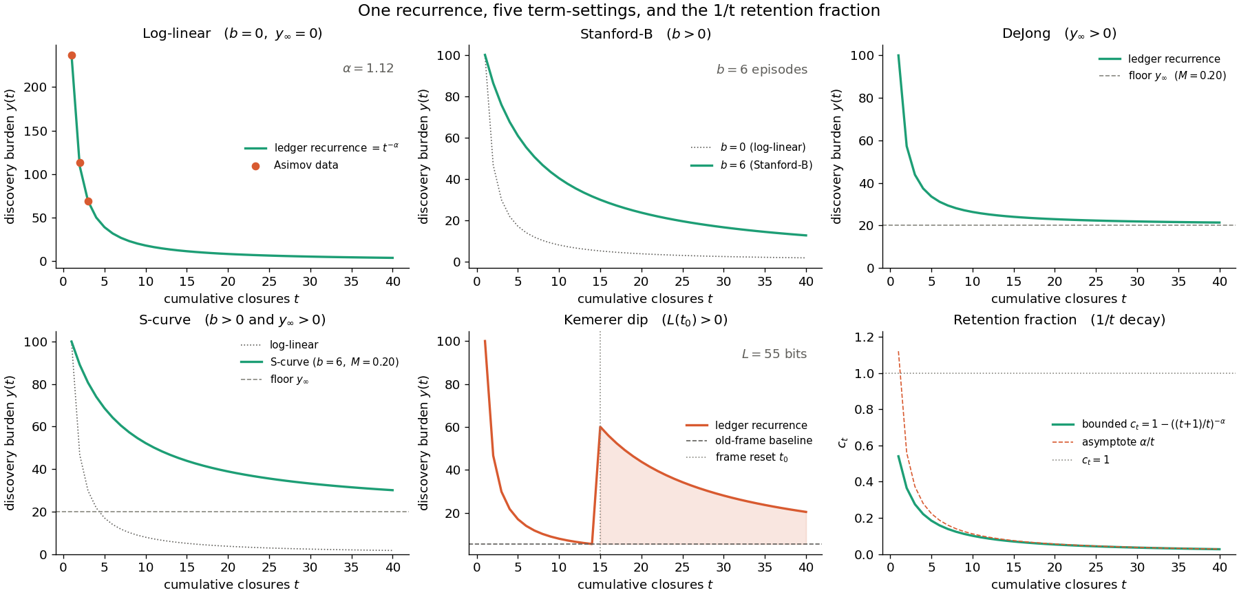
As multi-ledger compositions, two further shapes are structural relations among copies of the same recurrence: the Jaber–Glock dual-phase curve is a share-weighted superposition of two sub-frame ledgers with distinct exponents, and the group curve is a frame-conditioned aggregate of individual ledgers coupled by a cross-learner transfer term. The catalogue is not a list of rival equations but a coordinate chart on one ledger — and a partly redundant chart, since Plateau and DeJong name a single floor.
6. From Latent Bits to the Observed Cost Curve
Sections 3–5 derive a curve in the information-theoretical currency. The ordinate is , latent bits of residual ignorance; the literature plots cost or effort per unit. This section connects the two through the operational one-bit effective-depth estimator, so the unification is anchored to a measurable quantity rather than to an unobservable entropy.
6.1 The operational estimator
Over a window of comparable episodes, the effective one-bit net estimator reads the per-closure residual ignorance off the execution ledger:
with the counted channel capacity and the surviving closures. Both are counts, not entropies. Theorem 2 of the prior work brackets the latent residual ignorance by this observable up to a calibration error and a sub-one-bit coding gap:
So the ledger recurrence in is observable, per window, as an effective action-units-per-closure ratio, within a bounded envelope.
6.2 Why the count ratio is the effort curve
The classical ordinate is effort per unit — action units expended per delivered unit. The estimator's numerator is effective discriminating work and its denominator is delivered units, so
The literature's is a fitted proxy for exactly this ratio; the ledger supplies its generative law and the calibration theory relating the fitted ordinate to bits.
6.3 KEDE: the normalized, unit-free ordinate
The classical curve is unbounded and unit-dependent — dollars, hours, lines of code — which is why the literature warns that a line of code means different things in different phases and that measurement can mask the curve entirely. KEDE removes both problems by the bounded transform
The latent counterpart is , and Corollary 2 pushes the Theorem 2 envelope through this transform, so the two differ by a controlled, mostly-observable amount. KEDE is therefore the learning-curve ordinate re-expressed on a common axis: a value near one means little remained to discover, near zero that most of the delivered work was discovery.
6.4 The derived curve in KEDE units
Substituting the power-law solution of Section 3 into the latent transform gives the learning curve in its normalized form:
Efficiency rises toward one as residual ignorance decays as a power of experience — a bounded, unit-free curve derived from the ledger and readable off delivery counts. Where the classical literature fits an unbounded cost curve and struggles with what its ordinate means across contexts, the ledger produces a bounded efficiency curve whose ordinate is the same quantity — missing knowledge — in every context.
6.5. Episodes, Windows, and Learning-Curve Observations
The knowledge ledger is episode-indexed, but the operational estimator is window-indexed. Theorem 2 of the prior work is stated for a window of comparable episodes: it brackets an average over the window, computed from a counted channel capacity and a count of surviving closures . The recurrence lives on ; the estimator lives on . Every empirical claim made in this paper is therefore a claim about a windowed ordinate, and the map between the two indices must be stated rather than assumed.
This is not a technicality imported by the ledger. The learning-curve literature is overwhelmingly windowed in its data and episodic in its rhetoric, and it almost never marks the transition. The ledger makes that visible, which is itself a contribution.
For instance, Baloff's automotive start-ups aggregate cost and output into production “lots” of fixed unit count, and his single-plant case uses monthly observations of average direct-labour hours per unit[10]. Ohlsson blocks Asimov's output into groups of one hundred books precisely because individual books are not comparable[1]. Kemerer's CASE data are project- and period-level accounting records[3]. Baloff and Becker, arguing against aggregation across learners, nevertheless recommend “averaging the values of the dependent variable over two or more trials” as a variance-reduction device for individual curves[6] — which is blocking. The abscissa is usually called cumulative output, but the observational unit is usually a block.
The operational measurement, however, is not defined directly on the hidden state . Under black-box observation we do not see the internal stages of an episode, we do not see the regulator's knowledge state , and we do not see the per-stage selection signals . What we observe is the externally visible execution channel: gross closure events, the generic action units between them, and the operational ledger that records which gross closures survive as net accepted closures inside an observation window.
Let be an observation window containing one or more episode indices:
The net accepted closures in that window are not merely the closures attempted or reported. They are the closures that survive the operational ledger:
The window-level operational estimates are therefore:
This means that a window-level should not automatically be read as the hidden per-episode state . It is an operational estimate over the selected window. Only in the special case where the window contains one comparable accepted closure does the window estimator approach an episode-level observation.
Implication for translating learning curves into the ledger
Every learning-curve translation must therefore declare its observation scheme. If , the curve is being observed at the episode level. If , the curve is a windowed average. If , the series is rolling and serially dependent.
The central rule is simple: learning happens across episodes, but black-box measurement happens through windows. The per-episode recurrence explains how residual ignorance changes from one closure to the next. The per-window operational ledger estimates how efficiently accepted closures were produced inside a chosen observation window. Conflating these two levels turns a useful learning-curve observation into a misleading claim about the hidden knowledge state of the learner.
6.5.1 Four windowing modes
Let a window be a finite set of consecutive closure indices in a fixed comparable task class. Four windowing conventions appear in the literature, and they are not interchangeable.
| Mode | Window | Where it appears | Effect on the derived curve |
|---|---|---|---|
| (a) Episodic | Wright unit curve; single-trial practice data | None; In this case, the operational estimate is closest to an episode-level reading:
|
|
| (b) Blocked | Fixed-count partition | Ohlsson's Asimov blocks; Baloff's production lots | Upward level bias, exponent preserved (Proposition W1) |
| (c) Rolling | Moving window of width | Monthly productivity reporting | As (b), plus boundary-dependent survival (§6.5.4) |
| (d) Expanding | Cumulative-average learning curve; machine-learning curves in training-set size | Exponent preserved only for ; intercept inflated (Proposition W2) |
Mode (a) has the lowest conceptual bias because it respects the per-episode recurrence. However, it usually has the highest empirical variance. Individual episodes may differ in local difficulty, disturbance realization, duration, context, and execution noise even when they belong to the same task class. For this reason, episode-level observations are best suited for derivation or for highly standardized work, but they may be unstable in field data.
Blocked windows (mode (b)) reduce variance by averaging over several closures, but they introduce temporal averaging bias. A block estimate should not be plotted as if it were the exact hidden state at the beginning or end of the block unless the analyst explicitly accepts that approximation. In the Asimov case, for example, the episodes are completed books, while the observations are blocks of books. The five observed points are therefore not five episodes; they are five blocked windows over many book-closure episodes.
Blocked windows are also where the aggregation problem becomes most important. If a block mixes different task classes, different learners, changing tools, changing quality bars, or different response-equivalence criteria, the resulting curve may describe the aggregation procedure more than the underlying learning process. The ledger response is to define the learner and the task class before counting. If the learner is an individual, the window must preserve individual comparability. If the learner is a group, the group may be treated as the black-box learner, but the curve should not then be interpreted as a simple average of individual learning curves.
Rolling windows (mode (c)) are useful for monitoring because they produce a smoother operational KEDE/KTD series. They are especially useful in software, services, and other knowledge-work settings where individual closures are noisy and where managers need a continuous signal. However, overlapping windows create serial dependence:
They also smooth and delay the visible effect of discontinuities. A tool-adoption dip, a forgetting event, a change in task class, or a reset in the response map may be partly hidden by the overlap. Thus rolling windows are strong for operational monitoring but weaker for identifying the exact functional form of a learning law.
Mode (d) deserves emphasis because the production literature carries two parallel conventions — the unit curve and the cumulative-average curve — that are routinely compared as if they were competing models of the same quantity. On the ledger they are one quantity read under two windowing conventions, and Proposition W2 gives the exact relation between them.
6.5.2 The window-averaging identity
The bridge between the two indices requires no new assumption, because the numerator and denominator of the estimator are both counts, and counts are additive over the episodes of a window. Let be the number of non-closure action units consumed by episode , let be the surviving closures of the window, and let be its invalidated closures.
Lemma W (window-averaging identity). Under A1 - A4, the net effective estimator of a window decomposes exactly as
where is the counted effective depth of surviving episode , and
Consequently, under the hypotheses of Theorem 2, the window estimator brackets the surviving-closure mean of the per-episode residual ignorance:
Proof. By Proposition 1 of the prior work the counted non-closure units of the window partition over its episodes, , while . Dividing gives the stated decomposition, which is an identity of counts and requires nothing beyond A1–A5. Applying the Theorem 2 envelope termwise to the surviving episodes and averaging yields the second display, since the envelope is uniform in and the calibration error and coding gap of a mean are the means of the respective errors.
Lemma W is the reason the episode/window distinction can be handled rather than merely deplored. The window statistic is an arithmetic mean of the very quantity the recurrence propagates, plus a non-negative debit for capacity consumed by closures that did not survive. Everything that follows is a statement about what averaging does to a convex, decreasing trajectory.
6.5.3 Blocked windows: level bias without exponent bias
Proposition W1 (block-averaging bias). Let the per-episode residual ignorance follow the power-law solution with , . Let with , write for the block midpoint, and let
Then:
-
Strict upward bias. for every .
-
Size of the bias. If , then
-
Exponent invariance. For a fixed-width blocking with midpoints ,
so a log-log regression across blocks recovers consistently; only the early blocks are displaced upward.
Proof. Claim (i) is Jensen's inequality: the block index set is symmetric about and is strictly convex on for every .
For (ii), write with . This index set has zero mean, zero third moment, and second moment . Taylor expansion about gives
Since , dividing by gives the stated ratio. Claim (iii) follows by taking logarithms and noting as .
The expansion in (ii) is asymptotic in and fails for the first block of an equal-count blocking, where . There the exact sum must be used, and the bias is not small. The table below evaluates the exact ratio for the blocking used in the Asimov reconstruction — five blocks of one hundred closures — at , the one-independent-example-per-closure case of §4.5.
| Block | Closure range | Midpoint | Exact | Asymptotic estimate |
|---|---|---|---|---|
| 1 | 1–100 | 50.5 | 2.62 | (invalid: ) |
| 2 | 101–200 | 150.5 | 1.040 | 1.037 |
| 3 | 201–300 | 250.5 | 1.014 | 1.013 |
| 4 | 301–400 | 350.5 | 1.007 | 1.007 |
| 5 | 401–490 | 445.5 | 1.004 | 1.004 |
The methodological consequence is sharper than a caveat. Under equal-count blocking the first block of a power-law learning curve is inflated by a factor that grows without bound as from below and diverges logarithmically at , while all later blocks are accurate to within a few percent. The first block therefore carries almost no information about the residual ignorance of the early episodes, and any parameter estimated primarily from it — most obviously the intercept and the Stanford-B offset of §5.1 — is correspondingly unstable. This is a ledger-side explanation for the familiar instability of first-unit cost estimates in the production literature, and it is the reason the Asimov figure must be read as a block average and not as the residual ignorance of any single early episode.
6.5.4 Expanding windows: when the exponent survives and when it does not
Proposition W2 (cumulative-average windowing). With define the expanding-window ordinate
Then, as :
-
Sub-critical case .
so the expanding-window curve is asymptotically parallel to the episodic curve in log-log coordinates, with the same exponent and a fixed level offset
-
Critical case .
so the offset diverges logarithmically and the local log-log slope is , approaching from above. The windowed curve appears flatter than the true curve at every finite .
-
Super-critical case . The sum converges, so
and the expanding-window exponent collapses to irrespective of . The exponent is not identified from a cumulative-average ordinate in this regime.
Proof. All three cases follow from the Euler–Maclaurin expansion of the partial sums of the Riemann zeta function. For ,
and for the partial sum is the harmonic number . Dividing by gives (i)–(iii). In case (iii) the leading term vanishes and the constant dominates.
Corollary W (ordinate-ratio identification of the exponent). Suppose the same episode sequence is reported under both the episodic and the expanding-window convention, and . Then
is a consistent estimator of the exponent that uses only the levels of the two ordinates at a single , with no regression and no differencing.
That is a known empirical regularity in the production literature, and here it drops out of the ledger as an averaging artefact rather than a substantive difference between two models. It also means the ordinate convention is identifiable: given both curves, their offset ratio estimates independently of the slope.
Corollary W supplies a consistency check the learning-curve literature does not currently have. Where both conventions are reported — which is common in production settings, since unit and cumulative-average curves are often tabulated side by side — the exponent implied by their level ratio can be compared against the exponent fitted from either slope. Disagreement is evidence that the comparability frame of §2.1 has failed somewhere in the series, since under a single frame Proposition W2 forces the two to agree.
Proposition W2 also bears directly on the mechanism of §4 as a consistency check. Amari's expected entropic residual is the marginal loss of the next example at evidence level : it is episodic in the evidence clock, not cumulative. The cumulative log-loss of the same process is
which is exactly Proposition W2(ii). The logarithmic factor separating the marginal from the cumulative learning curve at the critical exponent is therefore not an artefact introduced by the windowing analysis; it is a standing feature of the setting from which §4 borrows, here re-derived from the ledger. The agreement is evidence that the window apparatus and the effective-evidence mechanism are describing the same object under two reporting conventions.
The critical case is in any event a boundary rather than an empirical regime. The classical learning rate per doubling is , and the production literature reports rates clustered between 80 and 90 per cent, which corresponds to
The critical exponent would require a 50 per cent learning rate, which is essentially unobserved in production settings. Sub-critical case (i) therefore governs the data actually available, and the entire impact of expanding-window reporting on such series is a fixed level offset of between roughly 1.18 and 1.47, with the exponent untouched.
Three places nevertheless require care. First, any curve imported from the literature under the cumulative-average convention must be corrected by before its intercept is compared with an episodic one. Second, machine-learning generalization curves — the row so labelled in the Appendix — are natively mode (d) in training-set size, so the marginal-versus-cumulative distinction is load-bearing for any future extension of the ledger in that direction. Third, and most consequentially for this paper, a process genuinely at or near the critical exponent, read under a cumulative-average ordinate, has local log-log slope — approximately at and at . A slope that steepens with accumulated experience is precisely the signature that invites an S-curve or a floor-plus-shift fit. The risk is therefore not to the derivation of §4 but to the perturbation readings of §5.3: a windowing artefact could be misattributed to a positive and a positive . Declaring the windowing mode is what forecloses that misreading.
6.5.5 Gross versus net closures and the settling lag
The second ambiguity is not about which episodes are averaged but about which are counted at all. Under black-box observation we do not see the internal stages of an episode, the regulator's knowledge state , or the per-stage selection signals . What we see is the externally visible execution channel — closure events and the generic action units between them — together with the operational ledger recording which gross closures survived as net accepted closures inside the window. The learning-curve literature has no counterpart convention. Scrapped units, defect rework, reverted changes, and abandoned projects are handled inconsistently or not at all.
Two consequences follow, and both are quantitative rather than rhetorical.
First, the choice of denominator determines whether yield improvement is visible as learning at all. Writing for the survival ratio, the two ordinates are related by . A gross denominator counts attempts rather than accepted closures, and improving yield does not reduce effort per attempt; only the net denominator registers a falling invalidation load as improvement. Gross counting therefore hides part of the learning and the fitted exponent is attenuated. In the limiting case where all improvement is yield improvement, a gross ordinate registers no learning whatsoever. Proposition I2 of §7.4 states the effect precisely and shows that a gross ordinate can even fall below zero, placing it outside the admissible range of a Knowledge To Be Discovered estimator. Because the attenuation is concentrated in the early episodes, it opposes the block bias of Proposition W1 on the same region of the curve, and the two cannot be separated from a blocked gross series alone. This means the two early-region biases now point in opposite directions. For instance, capacity 100, fifty attempts per window throughout, 25 surviving early and 50 late. Net ordinate goes 3 → 1. Gross ordinate goes 1 → 1: no learning visible at all.
Second, survival is a window-relative judgement. A closure accepted at and invalidated at belongs to under one window boundary and to under another, so depends on where the window is closed in a way that does not. This is arguably the sharper wedge. The episode/window question is about bias in the ordinate; the gross/net question is about what is being counted at all, and no learning-curve model in the literature specifies it.
We therefore adopt an explicit convention.
Convention S (settling lag). Fix a settling lag in closure units. A gross closure occurring at is counted in if and only if it has not been invalidated by . A window is read only after its last episode has settled. The reported ordinate is then a function of , and must be reported alongside it.
Convention S makes blocked windowing the natural default and rolling windowing the least safe: a rolling window whose stride is shorter than will count the same closure as surviving in one window and invalidated in the next, producing spurious non-monotonicity that has nothing to do with the loss term of §5.4. The adoption dip and the settling artefact are visually identical; only a declared distinguishes them.
6.5.6 Two axes of aggregation
Section 2.1 read Baloff and Becker's futility result as a statement about comparability frames. The window apparatus now lets us state it more precisely, because there are two distinct aggregation operations in play and the literature conflates them — including in Baloff and Becker's own paper, whose argument concerns one axis while whose proposed remedy operates on the other.
Remark (separation of the two axes).
-
Temporal aggregation pools episodes of one learner within one comparability frame. It is always admissible, because by Lemma W it is an operation on the estimator: counts are additive, so the window statistic is an exact mean of per-episode depths. Its cost is the level bias of Proposition W1 and the shape distortion of Proposition W2, both of which are computable and neither of which changes the exponent in the sub-critical regime.
-
Cross-learner aggregation pools ledgers of different learners. It is an operation on the state, not the estimator. By the argument of §5.6, the aggregate obeys a recurrence with the share-weighted effective retention
which is not constant even when every is. Functional form is therefore preserved only when the individual retention laws coincide — the equal-parameter condition Baloff and Becker identify and rightly decline to assume.
The separation resolves the apparent tension in their paper. Their objection is to axis (2), and it is correct: aggregating heterogeneous ledgers changes the equation. Their remedy — averaging the dependent variable over two or more trials — operates on axis (1), and it is also correct, because temporal blocking preserves the exponent. The two moves are compatible because they act on different objects: one on the estimator, one on the state. Nothing in the ledger licenses reading a group curve as an individual curve; everything in it licenses reading a block average as a windowed individual curve.
6.5.7 Convention adopted in this paper
Nothing in the literature counts N. The ordinate is cost or time, never capacity-over-closures. That's precisely why the Asimov -calibration is needed, and why it should be stated as a general protocol: any published curve can be converted, but only by importing a capacity convention the original authors never supplied. The conversion is therefore an interpretation of their data, not a re-reading of it.
Unless stated otherwise, the following convention is used throughout.
- The observational unit is a fixed-count blocked window with a declared settling lag under Convention S.
- The reported ordinate is the net effective estimator , or its bounded transform , never a gross-output ratio.
- Block statistics are plotted against the block midpoint , not the block endpoint, and the first block of any equal-count blocking is excluded from intercept estimation by Proposition W1.
- Where an expanding-window ordinate is taken from the literature, the level correction of Proposition W2 is applied before comparison with an episodic ordinate, and the super-critical case is flagged as non-identified.
With this convention fixed, the derivations of Sections 3–5 may be read as statements about while remaining testable against windowed data, and the Applications section's Asimov reconstruction acquires its correct status: a blocked-window estimate whose first block is inflated by a known factor, not a per-episode measurement.
7. What the Observed Ordinate Can and Cannot Determine
Sections 3–5 derive trajectories in the latent ordinate , and Section 6 connects that ordinate to a counted estimator. Between the two lie three conventions, each of which the practitioner must choose and none of which the learning-curve literature routinely reports: a measurement convention supplying the action unit and hence the coding gap, a windowing convention supplying the observational unit, and a counting convention supplying the rule by which gross closures become net closures.
This section asks what survives the composition of the three. The answer is not uniform. One parameter of the derived curve is identified and can even be estimated by a route the literature does not currently use; one is biased in a signed and computable way; and one is not identified at all below a resolution threshold, so that a published value of it may be entirely an artefact of the measuring instrument. Since the catalogue of Section 5 distinguishes its members precisely by these parameters, the result bears directly on the question of which learning-curve models can be told apart from data.
7.1 The composed observation model
Write the three layers explicitly. At the measurement layer, Theorem 2 of the prior work gives, for each surviving closure,
The calibration error is signed and, in principle, estimable; the coding gap is one-signed and bounded by a single action unit per closure. At the windowing layer, Lemma W averages these over a block. At the counting layer, the analyst chooses whether the denominator is or . The reported ordinate of block is therefore
where is the identity under net counting and the yield distortion of §7.4 under gross counting. The structural object of interest is the four-parameter family of Section 5,
We ask, for each component of , what the sequence determines.
7.2 What is identified: the exponent
The exponent is the robust parameter of the family, and it is robust for a structural reason: it is a property of the ratio of successive ordinates, whereas all three conventions contribute additive or multiplicative level terms that either vanish asymptotically or cancel in differences.
Three results already established combine to give this. Proposition W1(iii) shows that fixed-count blocking leaves the log-log slope intact, with block-level distortion vanishing in the block index. Proposition W2(i) shows the same for expanding windows in the sub-critical regime, where only the intercept moves. And the additive envelope is bounded while is not, so on any range where the envelope is a vanishing relative perturbation of the slope.
Two qualifications are essential, and they are the two negative results of §7.3 and §7.4 seen from the exponent's side. The envelope argument fails precisely where the curve approaches its floor, which is where the exponent and the floor trade off against each other in a fit; and the counting layer attenuates the slope whenever yield is improving. The exponent is therefore identified on the region of the curve where residual ignorance is large relative to one action unit per closure, under net counting, and only there.
Corollary W of §6.5.4 adds a second, independent route. Where a series is reported under both the episodic and the cumulative-average convention — the unit curve and the cumulative-average curve of the production literature — the exponent follows from the level ratio of the two ordinates at a single point, with no regression. Because that estimator uses levels rather than slopes, its bias profile is different from the regression estimator's, and disagreement between the two is diagnostic: under a single comparability frame Proposition W2 forces them to agree.
7.3 What is not identified: the floor
The floor is the parameter that distinguishes DeJong and Plateau from log-linear, and the combination of floor and offset that distinguishes the S-curve from both. It is also the parameter that the measurement layer is least able to determine, because a persistent coding gap is observationally indistinguishable from a persistent epistemic floor.
Proposition I1 (floor–gap non-identification). Suppose the observed ordinate converges, , with and . Then the latent floor satisfies
and the identified set for given the observed asymptote alone is the interval
In particular, if
then : the hypothesis of no epistemic floor cannot be rejected, and the fitted DeJong or Plateau constant may be entirely an artefact of the action-unit resolution.
Proof. Taking limits in the composed observation model gives the first display. The map
is not injective on ; its fibre over projects onto the stated interval in the first coordinate, since may take any value in and any value in its bound, subject to .
The consequence for Section 5.2 is immediate. The normalized incompressibility factor inherits the non-identification in its numerator and, by §7.5, additional width in its denominator. A reported is therefore an upper bound on the epistemic incompressibility of the task, never a point estimate, unless the observed asymptote exceeds one action unit per closure by more than the calibration bound. This does not affect the algebra of §5.2 — the DeJong form is still the floor perturbation of the recurrence — but it means that fitting DeJong rather than log-linear is not, by itself, evidence that an epistemic floor exists.
Non-identification here is a resolution limit rather than a permanent obstruction, and the ledger says how to lift it.
Corollary I1 (identification by unit refinement). Fix a reference action unit and measure the same process at the refined unit , . Expressed back in reference units, the observed asymptote is
so the coding-gap contribution to the identified set shrinks at rate and
An epistemic floor is therefore identified, up to calibration error alone, in the limit of action-unit refinement.
Corollary I1 converts a caveat into a test. A genuine frame-relative floor, in the sense of §5.2, is a property of the task frame and is invariant under refinement of the counting unit; it responds instead to frame interventions — adding a sensor, supplying the missing work instruction, refining the response-equivalence map. A coding gap is the opposite: it is invariant under frame intervention and shrinks under unit refinement. The two therefore have orthogonal comparative statics, and either intervention discriminates them:
| Intervention | Genuine epistemic floor | Coding gap |
|---|---|---|
| Refine action unit | unchanged | falls as |
| Refine frame (add information channel) | falls; new curve begins | unchanged |
Neither intervention is available retrospectively for a published curve, which is the honest conclusion: the epistemic floors reported in the historical literature are not recoverable from the published ordinates. They are recoverable prospectively, from a process instrumented to permit unit refinement.
7.4 What is biased: the counting layer
The third convention concerns which closures enter the denominator. Let
be the survival ratio of episode , and let denote the estimator computed with the gross denominator.
Proposition I2 (yield attenuation). With held fixed,
Consequently:
-
Domain violation. , with strict inequality whenever , and whenever . The gross ordinate is thus not an admissible estimator of Knowledge To Be Discovered: it can leave the non-negative range.
-
Slope attenuation. Where the ordinates are differentiable in ,
If yield improves with experience, , the second term is non-negative and the gross slope is strictly less steep. The fitted exponent is therefore attenuated: . The sign reverses if yield deteriorates.
-
Transience. If with , , then
so the attenuation vanishes asymptotically and is concentrated in the early episodes.
Proof. The identity is immediate from and . Claim (i) follows since , and the stated threshold is where the right-hand side falls below one. Claim (ii) is the logarithmic derivative of the identity. Claim (iii) is direct differentiation.
The direction deserves emphasis, because the intuitive expectation runs the other way. One might suppose that a gross ordinate credits declining scrap to learning and so overstates the exponent. The opposite holds. A gross denominator counts attempts, and improving yield does not reduce effort per attempt; it is the net denominator that registers yield improvement as improvement. Gross counting therefore hides the yield component of learning rather than inflating it.
A numerical illustration makes this concrete. Suppose the window capacity is action units throughout, and that the process makes fifty attempts per window in both an early and a late window, of which twenty-five and fifty respectively survive. Then
a threefold reduction in residual ignorance, whereas
so the gross ordinate registers no learning whatsoever. All of the improvement in this example is yield improvement, and gross counting is blind to it.
A second consequence matters for diagnosis. Proposition W1 inflates the early blocks of a blocked series, while Proposition I2 deflates the early points of a gross series. On blocked gross data the two act in opposite directions on the same region of the curve, and the fitted exponent is a mixture whose components cannot be separated without either the block-level raw counts or an independently reported yield series. A gross blocked curve that appears well behaved may therefore be two substantial biases in partial cancellation, and the apparent absence of distortion is not evidence of its absence.
7.5 What is weakly identified: intercept and prior-experience offset
The remaining parameters, and the Stanford-B offset , are determined mainly by the early part of the curve, which is exactly where every distortion catalogued above is largest: the block bias of Proposition W1 is and diverges as the first block is approached; the yield attenuation of Proposition I2 is concentrated there; and the frame is least likely to have stabilized.
Moreover and trade off against each other directly: over any finite range,
for a one-parameter family of pairs, the approximation improving as the observed range moves away from the origin. This is the ledger-side account of a well-known practical difficulty: first-unit cost estimates in the production literature are notoriously unstable, and the Boeing and Pierson estimates of carried-over experience are reported as ranges — one to ten airframes, one to six months — rather than as point values. Under §5.1 those ranges are estimates of a prior-experience offset, and Proposition W1 explains why the range is wide: the block that would determine it is the block least able to.
The practical recommendation of §2.2.7 follows directly. Exclude the first block of an equal-count blocking from intercept and offset estimation, and report as an interval.
7.6 Summary
| Parameter | Catalogue role | Status | Governing result | Remedy |
|---|---|---|---|---|
| log-linear slope; learning rate | Identified where , under net counting | W1(iii), W2(i) | — | |
| (second route) | as above | Identified from level ratio of two ordinate conventions | Corollary W | consistency check on the regression estimate |
| (gross data) | as above | Attenuated, signed by | I2(ii) | net denominator with declared settling lag |
| (expanding window, ) | as above | Not identified; collapses to 1 | W2(iii) | use episodic or blocked ordinate |
| , | DeJong factor; Plateau constant; S-curve asymptote | Not identified when | I1 | unit refinement (I1 corollary); frame-perturbation test |
| , | first-unit cost; Stanford-B carried-over experience | Weakly identified; mutually confounded | W1(ii), I2(iii), §7.5 | drop first block; report as interval |
7.7 A reporting protocol
The results above are negative only in the absence of metadata that costs nothing to record. We therefore state the minimal reporting protocol under which a learning curve becomes interpretable on the ledger.
- The action unit and how it was fixed — externally, or by calibration to a best observed window.
- The windowing mode (a)–(d) of §2.2.1 and, for blocked or rolling modes, the block width and the plotting abscissa (midpoint or endpoint).
- The counting convention, gross or net, and the settling lag of Convention S.
- The survival ratio series , or at minimum its endpoints, so that Proposition I2 can be inverted.
- Whether the frame was revised during the observation window, and where.
Items 1–4 are sufficient to convert a published curve into a ledger ordinate with a stated identified set for each parameter. Their absence, not any deficiency of the underlying data, is what makes the historical corpus only partially recoverable.
7.8 Consequence for the catalogue
Section 5 demoted the learning curves catalogue from a menu of rival equations to a coordinate chart on one recurrence. The present section constrains how much of that chart is legible from data.
The distinction between log-linear and DeJong or Plateau turns entirely on , which Proposition I1 shows is not identified below one action unit per closure. The distinction between log-linear and Stanford-B turns on , which §7.5 shows is weakly identified and confounded with the intercept. The S-curve requires both. Only the exponent, which all four share, is securely determined. It follows that a substantial part of the model-selection literature — the comparison of residuals that decides which of the fifteen equations a dataset prefers — is adjudicating between parameters that the reported ordinate does not determine.
This suggests a reading of the meta-analytic evidence more specific than the one offered in §8.1. Grosse and colleagues report that different curve families win for different datasets. Part of that variation may be substantive, reflecting which ledger terms are active in which task class. But part of it is predicted here to be conventional: datasets reported on a cumulative-average ordinate, on gross output, or with coarse action units should systematically favour different members of the catalogue than the same processes measured otherwise, irrespective of the underlying learning. The prediction is testable wherever the source studies document their measurement protocol, and it is falsifiable in the useful direction — if observational convention turns out to carry no explanatory weight in the meta-analytic sample, the identification results below remain valid as bounds but lose their claim on the historical record.
We state it as a prediction rather than a finding. Recovering the measurement protocol of several hundred published curves is a distinct undertaking, and nothing in Sections 3–6 depends on its outcome.
8. Discussion
8.1 What the derivation buys
Three things follow from reading the learning curve as ledger dynamics rather than fitting it.
First, the curve's shape is explained, not assumed. The log-linear form is the solution of the knowledge-ledger recurrence under one retention law, and the exponential is the solution under another. The power-law-versus-exponential question — which Ohlsson settles for Asimov by comparing log-log and semi-log residuals — becomes a question about a single structural quantity, the retained fraction , rather than a contest between two curves. Section 4 gives one sufficient reason holds under stationary redundant sampling.
Second, the literature's catalogue of fifteen equations is demoted from a menu to a coordinate chart. Stanford-B, DeJong, and the S-curve are one solution under three parameter settings, and their classical constants acquire bit-valued meanings: carried-over experience is stored coupling, the incompressibility factor is irreducible entropy, the adoption dip is a loss-bearing frame reset. The meta-analytic finding that different curves win for different data — Grosse and colleagues report the S-curve best for a large share of time-reduction datasets and exponential models best for others — is on this reading not a competition between theories but a report of which parameters are active in which task class.
Third, the ledger uses the axis the empirical literature wants. Both Kemerer and the literature argue that cumulative output, not calendar time, is the correct abscissa, and that measuring against time is a source of the contradictory CASE evidence. The ledger is natively closure-indexed, and the Knowledge Discovery Rate layer reattaches time separately through the unit convention. The predictive superiority Everett and Farghal report for the simpler log-linear and Stanford-B forms — better forecasts even when richer equations fit the past better — is consonant with a generative account: the log-linear form is the bare recurrence, and the extra parameters of the richer curves are the perturbations of Section 5, which help in-sample but overfit out-of-sample when their governing terms are inactive.
8.2 Where it breaks
The mechanism is sufficient, not necessary, and it is bounded by the comparability frame. Three limits matter.
The frame must hold. If , , or drift, Assumption E fails, each episode samples a partly new relation, and the ledger measures no single . The primer's own warnings — that a line of code means different things across phases, that seasonal and growth biases mask the curve — are exactly frame violations, and no derivation survives them. The theory locates the failure but does not repair it.
Retention need not dilute as . Non-stationary evidence, a growing reservoir , or interference between episodes give other laws and other shapes. The hyperbolic, Gompertz, and plateau forms that win for certain task types in the meta-analysis presumably correspond to such laws; deriving them is future work, not a claim of this paper.
Forgetting is only sketched. Section 5 reinstates as a one-time reset to produce the Kemerer dip, but sustained forgetting — a positive at every episode — would compete with retained gain and could halt or reverse the curve. The ledger accommodates this term but this paper does not solve the resulting dynamics.
8.3 What is claimed
The claim is narrow and, we think, defensible: under a stable task class sampled redundantly, the knowledge-ledger recurrence reproduces the log-linear learning curve, with the exponential as the special case in which cross-episode redundancy is ignored, and with Stanford-B, DeJong, and the Kemerer dip as perturbations of the same equation. The empirical curve is thereby exhibited as a consequence of knowledge-discovery accounting rather than as a free-standing regularity. What remains open — whether is also necessary, and which laws generate the non-power-law shapes — is the natural continuation.
9. Conclusion
The learning curve has been, for nearly a century, a regularity in search of a mechanism: measured everywhere, fitted routinely, derived nowhere. This paper supplies one mechanism. The closure-indexed knowledge ledger obeys an exact stock-flow identity, and read as a difference equation in the per-episode residual ignorance , that identity generates the learning curve rather than presupposing it.
The result is a single quantity governing the whole family. When the fraction of residual ignorance retained per episode is constant, the recurrence decays exponentially; when it dilutes as , it follows the power law — the log-linear curve . The power-law-versus-exponential debate, long adjudicated by comparing residuals, is thereby recast as a statement about how retention scales with experience, and Section 4 gives one sufficient reason — stationary redundant sampling of a fixed task relation — for the diluting case to hold.
Around that core, the primer's catalogue resolves into one solution under four settings of two terms: log-linear, Stanford-B with carried-over coupling shifting the origin, DeJong with irreducible entropy lifting the asymptote, and the Kemerer adoption dip with a loss-bearing task-class reset. Classical parameters become bit-valued quantities, and the KEDE transform re-expresses the whole curve on a bounded, unit-free axis whose ordinate — missing knowledge — means the same thing in every context, with the operational estimator tied to the latent quantity through the Theorem 2 envelope.
The claim is deliberately bounded. We show that dilution is sufficient to derive the log-linear curve, not that it is necessary, and the account holds only where the comparability frame holds. What lies beyond — whether the diluting law is also forced, and which retention laws generate the hyperbolic, Gompertz, and plateau shapes that other task classes prefer — is the natural continuation of this line. But the central point stands: the learning curve is not a free-standing empirical law to be catalogued. It is what knowledge-discovery accounting looks like when a stable task is practiced, and its most familiar form is one equation of one ledger.
Applications
The Knowledge-Centric Perspective builds on Ashby's Law of Requisite Variety by emphasizing that successful outcomes depend not only on a system's range of possible responses, but also on its ability to select the right response for each disturbance. This requires internal “system knowledge” that maps disturbances to appropriate actions. As Francis Heylighen proposed in his “Law of Requisite Knowledge,” effective regulation demands more than variety—it demands informed selection[29]. This knowledge-centric lens provides a foundation for analyzing how systems—biological, technical, or organizational—achieve control not just through options, but through understanding. The model we present operationalizes this perspective by estimating the informational requirements a system must satisfy to achieve its observed level of regulatory performance.
In what follows, we apply this Knowledge-Centric Perspective to a range of domains, including motor tasks and manual assembly, industrial assembly lines, software development processes, speed of light in a medium, intelligence testing and sports performance. In each case, the model enables us to estimate, in bits of information, the amount of knowledge a system must lack to produce its observed level of performance. By quantifying the knowledge to be discovered H(X|Y), we assess how much uncertainty was there in the system's ability to select appropriate responses. This allows us to compare systems not by tangible outcomes, but by the hidden knowledge structures required to achieve them, offering a unified lens for analyzing adaptation, skill, and control across diverse contexts.
Anchoring KEDE to Natural Constraints
In our model, N is always the theoretical maximum action rate (selections + outcomes) in an unconstrained environment, and S is the observed outcome rate under specific conditions over a given interval.
A key question is how to assign a natural constraint to N. That is, what constitutes an appropriate reference value for the maximum action rate (selections + outcomes)?
We may turn to physics for an instructive analogy. A quantum (plural: quanta) represents the smallest discrete unit of a physical phenomenon. For instance, a quantum of light is a photon, and a quantum of electricity is an electron. In this context, the speed of light in a vacuum serves as a fundamental upper bound for N. However, identifying an analogous natural constraint for human activity—particularly knowledge work—presents greater challenges.
Consider the example of typing. Here, the quantum can reasonably be defined as a symbol, since it is the smallest discrete unit of text. A symbol may be a letter, number, punctuation mark, or whitespace character. To determine the appropriate bin width Δt, we refer to empirical data on the minimum time required to produce a single symbol. Typing speed has been subject to considerable research. One of the metrics used for analyzing typing speed is inter-key interval (IKI), which is the difference in timestamps between two keypress events. We see that IKI is defined equal to the symbol duration time t. Hence we can use the research of IKI to find the symbol duration time t. Studies have reported an average IKI of 0.238 seconds [26], yielding a maximum human typing rate of approximately r=1/t=1/0,238=4.2 symbols per second
A similar approach can be applied to tasks such as furniture assembly. In this case, a plausible quantum is a single screw tightened, since it represents a minimal, repeatable unit of outcome. We then identify Δt as the average time required to tighten one screw. Empirical studies report that this task typically takes between 5 and 10 seconds[34]. Using the upper bound, we estimate the maximum screw-tightening rate as N=1/t=1/10=0.1 screws per second.
This methodology offers a principled way to estimate N using domain-specific quanta and empirically grounded time durations, enabling the application of our model to a broad range of human tasks.
The next question concerns the appropriate definition of outcome for measuring S and N.
Both N and S can always be discretized—or “binned”—in a way that preserves the total information rate, regardless of whether the outcome arises from natural processes, human behavior, or machines. By choosing a bin width Δt small enough (e.g., milliseconds), the range of possible tangible outcomes within each bin shrinks dramatically. This reduced range leads to less uncertainty in each bin, which compensates for the smaller time interval. Yet the ratio
remains an accurate measure of information rate.
As Δt becomes smaller, the measurements of S and N become more precise, as they reflect outcome over finer time intervals. But how small should Δt be? This dilemma is resolved by considering the granularity of outcomes associated with the outcome. The set E of outcomes can be thought of as the effects of the regulation process — the resulting states after the regulator responds to disturbances. In our model E is a sequence of {0,1}, where 0 = wrong outcome(failure to regulate) and 1 = acceptable outcome. So the presence of a concrete outcome leads to a natural binning of the outcomes, It also enables a clear distinction between signal (the entropy associated with producing the outcome) and noise (the residual variability unrelated to success or failure).
For example, two distinct symbols typed (e.g., ‘a' vs. ‘b') are clearly different outcomes. However, if one symbol is typed in 91 milliseconds and another in 92 milliseconds, this minute variation is inconsequential to the outcome. Such timing fluctuations are typically unintentional, irrelevant to task performance, and should not be considered part of the outcome. In practical terms, if the theoretical upper bound N is known—for instance, 4.2 symbols per second as derived from human typing speed, and the observed rate is S=1 symbol per second, then time should be partitioned into one-second bins. Each bin then yields a single outcome: either 1 (a symbol was successfully typed) or 0 (no symbol typed or incorrect input).
This binning principle generalizes beyond typing. Whether analyzing foot strikes in trail running (where negligible spatial change occurs over milliseconds) or the discrete moves in solving a Rubik's cube (where each turn resolves multiple potential states into a single action), binning ensures that no intermediate state need be modeled explicitly.
Physical applicability claim. For any isolated physical system to which a finite entropy bound applies, the number of physically distinguishable states is finite. Therefore the system admits a binary encoding whose length is bounded by the corresponding entropy bound expressed in bits. In holographic settings, this gives an upper bound of binary discriminations. Here they use the Planck length meters) and its associated surface area, the Planck area . Hence the Knowledge To Be Discovered Estimator applies to such physical systems after representing admissible states by a bounded sequence of binary discriminations.
Calculating Knowledge To Be Discovered from a Reported Learning Curve
Reported learning curves usually give time, cost, or speed as a function of accumulated practice. They do not directly report the internal selection trace of the actor. Nevertheless, if the repeated output can be interpreted as a sequence of closure acts, the learning curve can be re-expressed in Knowledge Discovery terms by defining the interval capacity from the best observed closure rate.
The demonstration below uses Ohlsson's data on Isaac Asimov's book-writing career[59]. The paper says Asimov wrote nearly 500 books over more than 40 years, treats one book as one practice trial, and groups the data into blocks of 100 books because individual books vary greatly in length and complexity. In that study, the completion of one book is treated as one completed knowledge-discovery episode. Therefore, for this reconstruction, one completed book is treated as one surviving closure.
Let denote block . Let be the number of surviving closures in the block, and let be the counted closure capacity of the same elapsed interval.
Under the time-normalized unit convention, counted capacity is defined by the elapsed duration of the interval divided by the selected unit length:
Learning-curve literature already treats the asymptote as the best possible performance limit[60]. At asymptotic performance, the actor still performs work, but no longer pays the earlier knowledge-discovery penalty. In many published learning curves, the asymptote is not directly known. Ohlsson’s Asimov paper is exactly like this. Ohlsson states that, after mastery, the tail of the curve approximates a horizontal line, and the asymptote represents the best possible performance. For this reconstruction, the unit length is not taken from an external physical limit. It is calibrated from the best observed block in the reported learning curve. In Asimov's data, the best observed closure rate occurs in the fourth block: 100 books in 46 months. Therefore:
Equivalently, the empirical closure capacity rate is:
The capacity of each block is then calculated as the number of book-closures that could have been produced in that block's elapsed time if the process had operated at the best observed closure rate:
From the effective one-bit net estimator in equation (5), the inferred Knowledge To Be Discovered for each block is then:
And the corresponding operational Knowledge Discovery Efficiency is:
Calculation
| Block | Elapsed time | Surviving closures S(I) | Capacity N(I) | ||
|---|---|---|---|---|---|
| 1 | 237 months | 100 books | 515.22 book-closures | 4.152 | 0.194 |
| 2 | 113 months | 100 books | 245.65 book-closures | 1.457 | 0.407 |
| 3 | 69 months | 100 books | 150.00 book-closures | 0.500 | 0.667 |
| 4 | 46 months | 100 books | 100.00 book-closures | 0.000 | 1.000 |
| 5 | 42 months | 90 books | 91.30 book-closures | 0.014 | 0.986 |
Interpretation
This conversion reads the published learning curve as an empirical-capacity curve. The best observed block defines the empirical closure-unit length: months per book-closure. Earlier blocks are then interpreted relative to that later demonstrated capacity.
In the first block, the elapsed interval had an empirical capacity of approximately 515 book-closures, but only 100 surviving closures were produced. The inferred is therefore 4.152. In operational terms, this means that for each surviving book-closure, the process consumed enough elapsed capacity for approximately 4.152 additional non-surviving or pre-closure units of residual ignorance. By the third block, the same method gives The process still contains substantial residual ignorance, but much less than in the early career phase. By the fourth block, the observed process reaches the empirical capacity anchor, so by calibration.
Notice that KTD does not necessarily fall to zero in the final block. The final block produced 90 books in 42 months. At the best observed rate, that interval had capacity for approximately 91.30 book-closures. Therefore the final block has a small positive and . This is conceptually preferable to forcing the last observation to be the zero-KTD point merely because it appears last in the sequence.
Methodological caveat
This is not a direct measurement of Asimov's internal knowledge discovery process. It is a reconstruction from reported learning-curve data. The calculation assumes that completed books are comparable enough to serve as closure units and that the best observed block is a reasonable empirical estimate of book-writing action capacity. Differences in book length, genre, research burden, publishing process, and external constraints may also affect the observed rate. Therefore, the result should be read as learning-curve-calibrated, not as a direct ledger measurement of Knowledge To Be Discovered (KTD).
The demonstration nevertheless shows how published learning curves can be translated into Knowledge Discovery terms. A learning curve becomes a visible trace of declining residual ignorance: as knowledge accumulates, the number of capacity units consumed per surviving closure falls, and operational KEDE rises.
Appendix
Different learning curves
Not all learning curves are the same. Some are steep, some are shallow, and some have multiple phases. The shape of the curve can reveal different underlying processes, such as rapid initial learning followed by a plateau, or gradual improvement over time.
Understanding the nuances of different learning curves can help in designing better training programs and interventions. It can also provide insights into the cognitive and behavioral mechanisms that drive learning in various contexts.
This distinction matters because the same phrase is used for at least four different objects. In human practice and production economics, a learning curve usually plots the time, cost, error rate, or productivity of repeated work against repetitions, cumulative output, or accumulated experience. In machine learning, a learning curve usually plots generalization performance against training-set size. In neural-network training practice, the same phrase is often used for a training curve: the loss or objective value plotted against epochs, iterations, or optimization steps. Feature and complexity curves add a fourth object: performance plotted against the number of input features, model parameters, or some other measure of representational complexity.
| Object called a learning curve | Typical horizontal axis | Typical vertical axis | Primary question | Status in this paper |
|---|---|---|---|---|
| Human practice curve | Practice trials, repetitions, or completed episodes | Execution time, error rate, success rate, or speed | How does an individual improve through repeated performance? | Direct target of the scalar ledger recurrence |
| Production or experience curve | Cumulative output, cumulative projects, or accumulated experience | Unit cost, unit time, productivity, quality, or output rate | How does a stable process improve as experience accumulates? | Direct target of the scalar ledger recurrence, after measurement-frame conditions are fixed |
| Technology-adoption curve | Projects, calendar time, or adoption episodes | Relative productivity, cost, quality, or realized benefit | How does performance change when a new tool or process initially disrupts an old one? | Treated as a frame-reset and loss-bearing extension of the ledger |
| Machine-learning generalization curve | Training-set size | Expected test risk, generalization error, accuracy, or predictive loss | How does performance on unseen data change as more training examples are supplied? | Related but not identical; requires a separate interpretation of examples, hypotheses, and predictive uncertainty |
| Training or optimization curve | Epochs, iterations, gradient steps, or passes over data | Training loss, validation loss, objective value, or reward | How does an optimizer improve a model during training? | Outside the main derivation unless optimization steps are explicitly modeled as closure episodes |
| Feature or complexity curve | Number of features, dimensions, parameters, or model complexity | Risk, error, accuracy, or loss | How does performance change as representational capacity changes? | Outside the main derivation; may be modeled later as changing response variety rather than accumulated experience |
| Variance learning curve | Cumulative individual, team, or organizational experience | Performance variance, consistency, dispersion, or reliability | Does experience make performance more predictable, not merely faster on average? | Requires a second-moment extension of the ledger |
Machine-learning generalization curves have a different statistical object: expected performance on unseen samples as training-set size varies. A future extension can connect them to the ledger by treating training examples as evidence that reduces predictive uncertainty over response rules, but that requires assumptions about hypothesis classes, sampling, loss functions, and generalization error that are not needed for the practice/production derivation.
Training curves are also kept separate. A curve of training loss against epochs or gradient steps describes optimization dynamics, not necessarily accumulated task experience. It may improve because an optimizer has found better parameters, because the same data have been revisited, or because the objective has been reshaped. Those mechanisms can be analyzed informationally, but they are not the same object as a production curve indexed by closed work episodes.
Feature curves and complexity curves are likewise distinct. They ask what happens when the learner's representational variety changes, not what happens when a fixed task class is practiced. In the language of the present paper, they concern changes in the available response space or model class, whereas the main learning-curve recurrence concerns changes in stored coupling within a fixed frame.
What learning could also do (but we are explicitly excluding)
Not every form of learning improves regulation H(E|Y) in Ashby's sense. Other possibilities include:
-
Expanding action variety without selectivity
Learning might increase (more possible actions, tools, behaviors) without reducing .
- The system becomes more capable in principle
- But still does not know which action to take
- Regulation does not improve
This violates Ashby's requirement that variety must be constrained, not merely expanded.
-
Improving buffering instead of knowledge
Learning might increase buffering capacity (delay, slack, tolerance), so disturbances are absorbed without better action selection.
- Outcomes may improve
- But does not increase
- Regulation improves without learning the mapping
This is explicitly separated from knowledge in Ashby's extended formulation.
-
Changing goals or success criteria
Learning could redefine what counts as success .
- Apparent performance improves
- But the structural coupling (mapping) is unchanged
- Information-theoretically, nothing about need change
This is semantic drift, not cybernetic learning.
-
One-off adaptation without structural retention
The system may succeed through exploration without storing the result.
- Regulation succeeds this time
- Next encounter repeats the same uncertainty
- No accumulation of
This is regulation, not learning.
Cumulative Knowledge To Be Discovered
Using
Cumulative w.r.t. S
Choose a baseline > 0.
Define:
Key properties:
- → is concave in .
Domain: ∈ (0, N]. Since > 0 for , increases with (for ) and is finite as long as .
Useful normalizations:
Dimensionless form with :
Total cumulative up to completion S = N:
This can be thought of as the total knowledge-effort curve or “cumulative residual variety as a function of performance level” i.e. how much “knowledge work” has been consumed to reach performance level S.
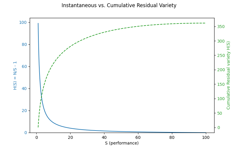
Fig.2 Total Knowledge-Effort Curve Here we see the cumulative residual variety as a function of performance level.
- Blue curve: instantaneous 𝐻(𝑆)=𝑁/𝑆−1H(S)=N/S−1 (residual variety ratio).
- Green dashed curve: cumulative residual variety C(S) as we accumulate uncertainty over growing performance level S.
How to cite:
Bakardzhiev D.V. (2026) Learning Curves: A Knowledge-Centric Perspective https://docs.kedehub.io/knowledge-centric-research/kede-learning-curves.html
Works Cited
1. Ohlsson, S. (1992). The Learning Curve for Writing Books: Evidence from Professor Asimov. Psychological Science, 3(6), 380-382.
2. L. B.S. Raccoon. 1996. A learning curve primer for software engineers. SIGSOFT Softw. Eng. Notes 21, 1 (Jan 1 1996), 77–86. https://doi.org/10.1145/381790.381805
3. Chris F. Kemerer (1992) How the Learning Curve Affects CASE Tool Adoption, in Software, Volume 9, Number 3, Pages 23 to 28, May 1992, IEEE Press
4. Grosse, Eric H. & Glock, Christoph H. & Müller, Sebastian, 2015. "Production economics and the learning curve: A meta-analysis," International Journal of Production Economics, Elsevier, vol. 170(PB), pages 401-412.
5. Viering, T., & Loog, M. (2023). The Shape of Learning Curves: A Review. IEEE Transactions on Pattern Analysis and Machine Intelligence, 45(6), 7799-7819. https://doi.org/10.1109/TPAMI.2022.3220744
6. Baloff N, Becker SW. On the futility of aggregating individual learning curves. Psychol Rep. 1967 Feb;20(1):183-91. doi: 10.2466/pr0.1967.20.1.183. PMID: 5341311.
7. Newell, A., & Rosenbloom. P.S. (1981). Mechanisms of skill acquisition and the power law of practice. In J.R. Anderson (Ed.), Cognitive skills and their acquisifion (pp. 1-56). Hillsdale. NJ: Erlbaum.
8. S. Amari, “Universal property of learning curves under entropy loss,” in IJCNN, vol. 2, 1992, pp. 368–373 vol.2.
9. S.-i. Amari, “A universal theorem on learning curves,” Neural Netw., vol. 6, no. 2, pp. 161–166, jan 1993
10. Baloff, N.,1971.Extensions of the learning curve—some empirical results. Oper. Res. Q. 22(4), 329–340.
11. Grosse, E.H.,Glock,C.H.,Jaber,M.Y.,2013.The effect of worker learning and forgetting on storage reassignment decisions in order picking systems. Comput. Ind. Eng.66(4),653-662.
12. H. Glock C, Y. Jaber M (2014), A group learning curve model with and without worker turnover. Journal of Modelling in Management, Vol. 9 No. 2 pp. 179-199, doi: https://doi.org/10.1108/JM2-05-2013-0018
13. Anzanello, M. J., & Fogliatto, F. S. (2011). Learning curve models and applications: Literature review and research directions. International Journal of Industrial Ergonomics, 41(5), 573-583.
14. Jaber, M.Y.,Glock,C.H.,2013. A learning curve for tasks with cognitive and motor elements. Comput.Ind.Eng.64(3),866-871.
Getting started