How to measure Organizational Scalability in software development
A knowledge-centric approach
Abstract
Most of today’s software projects are so complex that they cannot be developed by a single developer. Instead, teams of software developers need to collaborate. This raises a simple, yet important question: How does team size affect productivity?
This question is of significant importance not only for project management but also for achieving broader business and operational scalability. Scaling an organization involves expanding its capabilities and structures in a sustainable way to handle increased market demand, customer base, and operational complexity. We answer this question from a Knowledge-Centric perspective on software development defining both what productivity and team size are.
Software development productivity is a ratio between the outcome produced and the new knowledge discovered to produce that outcome. The outcome can be quantified in various ways, such as revenue or profit. Since the outcome is evaluated by the market, we assess scalability using the efficiency with which the knowledge was discovered. For that we utilize the Knowledge Discovery Efficiency (KEDE) - a metric designed to guide the optimization of software development , focusing on knowledge as the essential resource. We define the team of a project to consist of all contributing developers who have committed at least once over a certain period of time such as on a weekly basis. We calculate both efficiency and team size using a patented technology that analyzes source code in local clones of Git repositories.
Using the calculated efficiency and team size we can perform a temporal analysis on how team size affects efficiency and represent it in a graph. The input changes can lead to three types of proportional output: constant, increasing, or decreasing/diminishing returns to scale. Examples are available here.
In addition we calculate a Scalability Coefficient that measures he ability of an organization to sustain or increase its efficiency when adding people - i.e. its performance in terms of returns on scale. A positive Scalability Coefficient indicates that increases in team size are associated with proportional increases in efficiency, suggesting increasing returns to scale. The larger the coefficient, the stronger the positive impact of scaling up the team size on efficiency, which is beneficial for the organization. A negative Scalability Coefficient suggests that increases in team size lead to proportional decreases in efficiency, indicating decreasing returns to scale. A constant Scalability Coefficient indicates that efficiency increases in the same proportion as team size. Examples are available here.
We study a popular blockchain project named Solana. Our findings confirm the negative relation between team size and efficiency previously suggested by empirical software engineering research, thus providing quantitative evidence for the presence of both a strong Ringelmann effect and valid Brooks' Law.
Last but not least, we provide actionable guidance on how to positively affect efficiency when increasing team size. We believe that our methodology is useful for both engineering leaders and executives with software development cost models based on empirical data from software development repositories.
Scalability
One may naively assume that the efficiency of individual team members is additive, i.e., that, compared to the time taken by a single developer, a team of n developers will speed up the development time by a factor of n. However, from a Knowledge-Centric perspective this naive perspective misses out two important factors that can give rise to a non-additive scaling of productivity.
First, the collaboration of developers in a team can give rise to positive synergy effects, due to increase in total existing knowledge in the tean, which result in the team being more productive than one would expect from simply adding up the individual productivities of its members. If that happens, the average productivity per team member can be increased by simply adding developers to the team, a fact that has been related to Aristotle’s quote that “the whole is more than the sum of its parts”
On the contrary, the increase of team size could negatively affect productivity, and it has thus been discussed extensively in science and project management.
The question of how factors like team size influence the productivity of team members was already addressed by Maximilien Ringelmann [4] in 1913. His finding that individual productivity tends to linearly decrease with team size is known as the Ringelmann effect, which is studied extensively in social psychology and organizational theory. Ringelmann highlighted this with his renowned “rope pulling experiment” – he found that if he asked a group of men to pull on a rope together, each made less effort when doing so as part of the group than when tugging alone.
Ringelmann’s findings are backed up by the experiments of Bibb Latané et al, who studied the phenomenon known as "social loafing"[9]. A key experiment that showed that, when tasked with creating the loudest noise possible, people in a group would only shout at a third of the capacity they demonstrated alone. Even just (mistakenly) believing they were in a group was enough to make a significant impact on the subjects’ performance. The researchers claimed that When groups get larger, individuals experience less social pressure and feel less responsibility because their performance becomes difficult, or even impossible, to correctly assess amidst a crowd.
In software project management, a similar observation is famously paraphrased as Brooks’ law [5]. By claiming that “adding manpower to a late project makes it later” it captures that the overhead associated with growing team sizes can reduce team efficiency. Whether this is a law or “an outrageous simplification” as Brooks himself claimed, three sound factors underpin his point:
- New team members are not immediately productive as they need to get familiar with the code base, existing knowledge and what knowledge is missing. During onboarding time, existing members of the group may lose focus as they dedicate time and resources to training the newcomer. The new developer could even have a negative impact on productivity by introducing defects and thus rework.
- Personnel additions increase communication overheads as everyone needs to keep track of progress, so the more people in the team the longer it takes to find out where everyone else is up to.
- There’s the issue of limited task divisibility i.e. some work items are easily divided but others are not. That is illustrated by Brooks’s charming example that, while one woman needs nine months to make one baby, “nine women can’t make a baby in one month”.
Recent studies using massive repository data suggest that developers in larger teams tend to be less productive than smaller teams, thus validating the view of software economics that software projects are diseconomies of scale[1][2]. Despite using similar methods and data, other studies argue for a positive linear or even super-linear relationship between team size and productivity[3].
At the same time, there is significant confusion over the question which quantitative indicators can reasonably be used to measure the productivity of software development teams or individual contributors. In this work we use the Knowledge Discovery Efficiency (KEDE) for measuring developer efficiency[6].
How to achieve positive Returns on Scale
Since we consider knowledge as the primary resource in software development. Thus, to improve efficiency, we need to:
- Acquire enough of the primary resource, by recruiting people with knowledge, skills and experience.
- Ensure a match between the level of knowledge each individual possesses and the level of knowledge required to do a job. This would enable even junior developers to contribute on par with seasoned professionals. It's not about the years of experience, but about how efficiently individuals and teams can learn and apply new knowledge to maximize their potential.
- Establish an iterative process that aims to acquire new and missing knowledge. Achieving efficient knowledge discovery hinges on the effective utilization and management of organizational knowledge resources.
- Minimize the amount of waste of the primary resource. There are two primary sources of waste - rework and time spent on non-productive activities.
For the organization as a whole, the goal is to minimize the average missing information.
We should also consider the question of the optimal team size. Jeff Bezos, Amazon CEO, famously claimed that if a team couldn’t be fed with two pizzas it was too big. Agile standing has evolved its “7 ± 2” people rule for team size into “3-9 people” over the years, showing a growing recognition of the value of even the smallest teams.
To analyze the problem and explore different corner cases involving changes in the number of developers and their average efficiency, consider various scenarios and their potential implications. Here are some corner cases and considerations:
-
Case 1: Decreasing Number of Developers and Decreasing Average Efficiency
- Scenario: The number of developers decreases from one week to the next, and the average efficiency also decreases.
-
Possible Causes:
- Loss of Highly Knowledgeable Developers: If the individuals who leave are more knowledgeable than the remaining group, the average efficiency will naturally decrease.
- Environmental/External Factors: Changes in work conditions, morale, or increased cognitive load could reduce the efficiency of remaining workers, compounding the effect of losing experts.
- Random Variation: Particularly in small groups, the departure of a few individuals (regardless of their efficiency) can significantly sway the average.
-
Case 2: Decreasing Number of Developers but Increasing Average Efficiency
- Scenario: The number of developers decreases, but the average efficiency increases.
-
Possible Causes:
- Removal of Less Knowledgeable Workers: If those who leave have lower expertise than the average, then the remaining group's average efficiency will increase.
- Motivational Increases: The remaining group might increase their efficiency due to changes in team dynamics or as a response to the increased responsibility.
-
Case 3: Increasing Number of Developers and Increasing Average Efficiency
- Scenario: More developers join, and the average efficiency increases.
-
Possible Causes:
- Addition of Highly Knowledgeable Developers: New additions might be better trained or skilled, raising the overall average.
- Scale Efficiencies: Sometimes, larger groups can operate more efficiently due to better division of labor or team dynamics.
-
Case 4: Increasing Number of Developers but Decreasing Average Efficiency
- Scenario: The number of developers increases, but the average efficiency decreases.
-
Possible Causes:
- Incorporation of Less Knowledgeable Workers: New additions might be less trained or skilled, bringing down the average efficiency.
- Dilution of Focus: With more people, coordination issues may arise, potentially leading to decreased overall efficiency.
Scaling an organization involves expanding its capabilities and structures in a sustainable way to handle increased market demand, customer base, and operational complexity. In essence, organizational scalability requires a multi-faceted approach that addresses not just the increase in output or customers, but also the internal and external structures that support those increases. This holistic approach helps ensure that growth is not just rapid, but also sustainable and effective over the long term.
Methodology
We apply the Knowledge-Centric perspective on software development to explain how team size affects productivity in software development. This perspective treats knowledge as the fuel that drives the software development engine.
According to the Knowledge-Centric perspective on software development the primary resource in software development is the existing knowledge all team members possess.
Data Set
We study the scalability of software development teams by analyzing source code in local clones of Git repositories, as explained in detail in the U.S. Patent[7].
In the Git version control system the development history of a project consists of a tree of commits, with the first commit representing the root and each subsequent commit storing a parent pointer to the commit immediately preceding it. In this way, starting from the most recent commit of a project, the whole development history can be traced back by following the parent pointers.
More specifically, for each commit we consider:
- the SHA hash uniquely identifying the commit
- the name and email of the developer who authored the commit
- the time stamp of the commit (with a resolution of seconds)
- the list of files changed by this commit
- the diffs of all files changed by the commit, which allows to reconstruct the precise changes to the source code at the level of individual characters
- the parent pointer (SHA hash) of the preceding commit
Measuring Software Development Efficiency
Central to the knowledge-centric perspective on software development is the concept of the 'knowledge gap' - the difference between what a developer knows and what they need to know to effectively complete tasks. This gap directly influences developer's' work experience, talent utilization and productivity.
Bridging this knowledge gap is a dynamic process, defined as the Knowledge Discovery Process. A Knowledge Discovery Process transforms invisible knowledge into visible, tangible output.
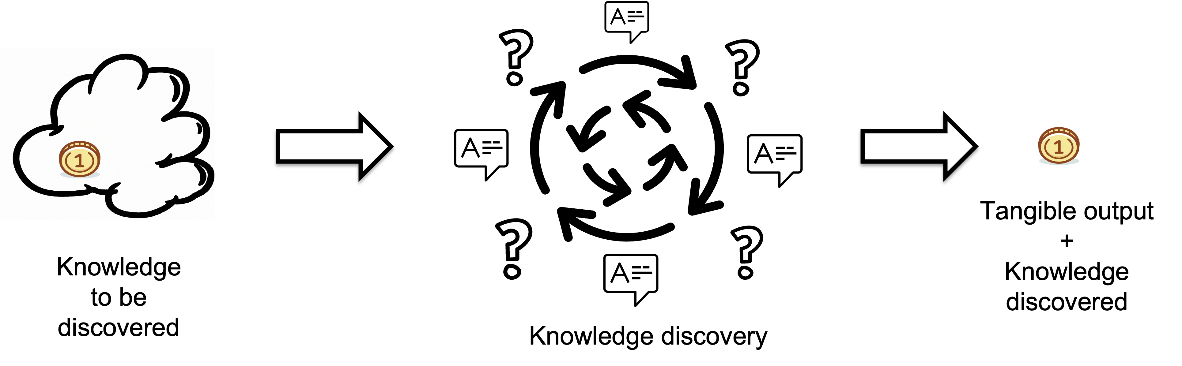
It is like a 'black box': its internal mechanisms may not be fully transparent, but the results it produces are clearly observable. To learn more about it, please refer to this article.
To explain the tangible output, we can use an analogy from physics where a quantum is the smallest discrete unit of a physical phenomenon. In software development, tangible output comprises symbols produced..The quality of the output is assumed to meet target standards.
Inputs represent the knowledge developers lack before starting a task i.e. the missing information or knowledge that needs to be discovered, which is measured in bits.
A crucial aspect of our approach involves measuring the knowledge gaps that developers bridge in completing tasks, quantified in bits of information. To quantify the knowledge developers didn't have before starting a task we use the KEDE theorem derived from the aforementioned principles:
(1)
Here, H denotes the amount of missing information in bits, N represents the maximum possible symbols that could be produced within a given time frame, h is the number of working hours in a day and CPH is the maximum number of symbols that could be contributed per hour. S is the actual number of symbols produced in that time frame, and W stands for the probability of waste.
We define N as the maximum number of symbols that could be produced in a time interval, assuming that the minimum symbol duration is one unit of time and is equal to the time it takes to ask one question.
Importantly, the KEDE theorem isn't tied to the absolute values of typing speed or cognitive capacity. Instead, it's based on the ratio between the manual work done and the manual work that could theoretically be done given the cognitive constraints. The value of N, or the maximum symbol rate, is used as a constant to represent an idealized, maximum efficiency over a standard work interval (such as an 8-hour workday). The specific values used for maximum typing speed and cognitive capacity are not the core components of the theorem itself; they are parameters that give context and allow for the application of the theorem to real-world scenarios. Changes in research would prompt adjustments in the constant N but would not necessitate a change in the structure or application of the theorem itself.
Next we introduce a new metric called KEDE (KnowledgE Discovery Efficiency).
Knowledge Discovery Efficiency (KEDE) is a metric designed to guide the optimization of software development , focusing on knowledge as the essential resource. KEDE quantifies the knowledge that a software developer lacked prior to starting a task, essentially measuring the knowledge they needed to gather to successfully complete the task. This knowledge gap directly influences developers' efficiency, impacting their happiness and productivity.
(2)
KEDE is a measure of how much of the required knowledge for completing tasks is covered by the prior knowledge. KEDE quantifies the knowledge software developers didn't have prior to starting a task, since it is this lack of knowledge that significantly impacts the time and effort required. KEDE is inversely proportional to the missing information required to effectively complete a task, and has values in the closed interval (0,1]. The higher the KEDE the less knowledge to be discovered.

- Minimum value of 0 and maximum value of 100.
- KEDE approaches 0 when the missing information is infinite, which is the case when humans create new knowledge, as exemplified by intellectuals like Albert Einstein and startups developing new technologies like PayPal.
- KEDE approaches 100 when the missing information is zero, which is the case for an omniscient being, such as God.
- KEDE is higher when software developers apply prior knowledge instead of discovering new knowledge.
- anchored to the natural constraints of the maximum possible typing speed and the cognitive control of the human brain, supporting comparisons across contexts, programming languages and applications.
For an expert full-time software developer who mostly applies prior knowledge but also creates new knowledge when needed, we would expect a KEDE value of 20.
Productivity
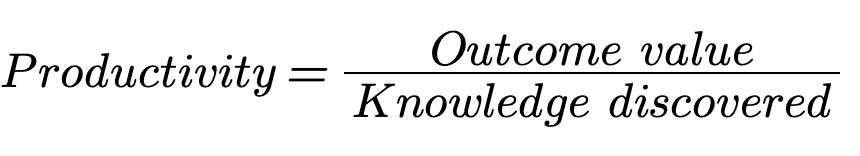
Software development productivity is a ratio between the outcome produced and the new knowledge discovered to produce that outcome. The outcome can be quantified in various ways, such as revenue or profit.
KEDEHub allows us to measure the amount of new knowledge discovered by our developers. This forms the denominator in the productivity formula.
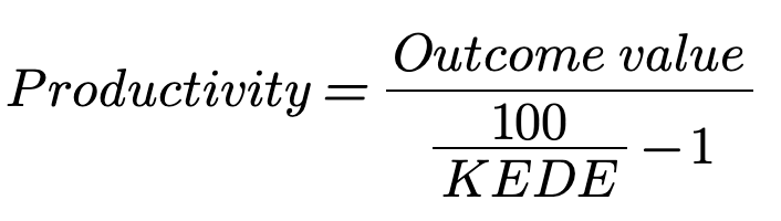
So, if the KEDE we measured is low, it means our developers needed a lot of new knowledge to produce the outcome. This might sound like bad news, but it's actually quite the opposite. It signifies that there's a lot of untapped human potential in our organization.
Measuring Team Size
Understanding the relation between team size and KEDE first requires a reasonable definition for the size of the development team. The simple question of who belongs to the development team of a corporate software project at a given point in time is not trivial to answer since one team could work on several projects. In case of an OSS project the simple question of who belongs to the development team is even more difficult to answer, because of the no “formalized” notion of who is a member of the project.
The Knowledge-centric perspective is a systems perspective, because it takes into account all of the behaviors of a system as a whole in the context of its ecosystem in which it operates. This includes team dynamics, organizational knowledge resources, development tools, and the overall work environment.
It's a common misconception to overestimate how much of the knowledge discovery efficiency is a function of the individual developers' skills and abilities and underestimate how much is determined by the system they operate in. Knowledge is a property of the organization the software developer operates in. This includes the knowledge of the developer, but also the knowledge of their teammates, the Product Owner, the architect, the QA, the support, the documentation available, the applicable knowledge in StackOverflow, and so on.
While it's true that designers, architects, and QAs may not produce code, they contribute significantly to helping developers produce code that meets customer expectations. Therefore, it's not recommended to measure the capability of individual developers. Instead, we should always measure the capability of an organization, whether that be a team, a project, or a company.
We are interpreting the team size (i.e., all developers that have committed in the productivity window) as the amount of resource available to a project.
Using time-stamped commit data, a first naive approach to define team size could be based on the analysis of activity spans of developers, i.e., taking the first and last commit of each developer to the project and considering them as team members in between the time stamps of those two commits. However, this simple approach generates several problems:
- Developers may leave the project, be inactive for an extended period of time and then rejoin the project later.
- The project might never finish, due to bug fixes or additional requirements. Thus, one-time contributors who - using this simple approach - will not be considered as project members even though they both contribute to the development
To avoid these problems we define the team of a project to consist of all contributing developers who have committed at least once over a certain period of time such as on a weekly basis. That is a rather restrictive definition for the size of the development team.
Temporal Analysis of Efficiency and Team Size
We expect a strong weekly periodicity in commit activity due to the effect of workdays and weekends. To ensure that this effect is equally pronounced in all time windows, we choose the window size of 7 days, We segment the commit history of each project in consecutive, non-overlapping productivity windows of 7 days. Accordingly we calculate KEDE for the same time interval e.g. per week. For each productivity window, we additionally calculate the number of active developers, i.e., the number of those developers committing at least once within a productivity time window.
We use the following procedure for an organizational unit and all of its projects:
- We first segment the history of the organizational unit into consecutive, non-overlapping windows of a certain size.
- For each productivity window we find the developers who have contributed and compute their total number
- After that, for each of the developers we aggregate their KEDE across all projects in the current productivity window.
Thus, for each productivity window we have:
- a list of all developers and for each developer their aggregated KEDE
- the number of developers who contributed
We can visualize the collected data as a time series and as a frequency chart.
As examples we shall look ate two diagrams where the result of the above procedure is applied to the case where:
- The organizational unit is a whole company. The company we will look into is Solana because their source code from the white paper and the first prototype through present days is publicly available.
- the productivity window is a week with a size of 7 days. Thus, we will consider aggregated Weekly KEDE.
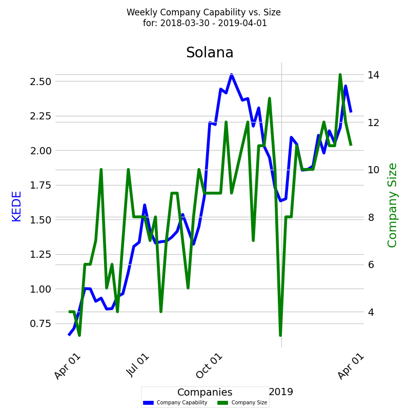
First a time-series.
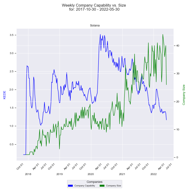
On the x-axis we have the quarter dates. Then we have two y-axises - one for the capability and one for the size of the company. Capability axis is to the left and is in Weekly KEDE values. How capability changes through time is presented by the dark blue line calculated using EWMA. Each point of the blue line is the average Weekly KEDE for all the developers who contributed in that week. Company size axis is to the right and is the number of developers who contributed to any of Solana projects in a given week. How company size changed through time is presented by the green line. Each point of the green line is the number of developers who contributed in a given week.
EWMA is calculated recursively using:
where span=10.
And then a frequency chart.
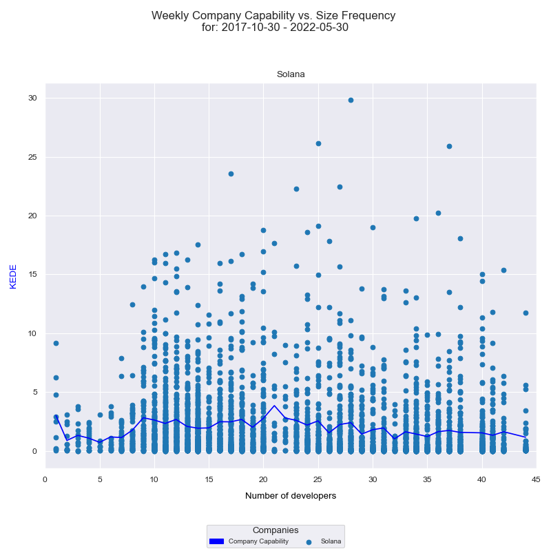
On the x-axis we have the number of developers who contributed to any of Solana projects in a given week. On the y-axis we have Weekly KEDE values. Each individual developer's aggregated Weekly KEDE is presented as a light blue dot on the diagram. The dark blue line is the average weekly KEDE for all developers calculated by arithmetic mean.
The first x-axis value is 1. For it there are six dots. Each dot is one contribution of the single developer who formed a team of one. Since we have six dots it means there were 6 weeks where the company size was of one contributing developer. There might have been more than one working, but only one contributed.
The last x-axis value is 44. We don't see at least 44 dots because they overlap.
For the x-axis values of 39 and 43 there are no dots. That means there wasn't a single week where 38 or 43 developers contributed.
Calculating the Scalability Coefficient
So far, our arguments about the scaling of efficiency with the size of the development team have been mostly visual. In the following, we substantiate these arguments by means of a regression analysis on Returns to Scale.
Returns to Scale is a concept from economics that measures how output changes in response to a proportional change in all inputs. It's particularly relevant in production and cost analysis, where we're assessing how scale impacts productivity. Understanding returns to scale might help us determine the relationship between team size (an input) and productivity (output) in a broader economic context.
There are three primary types of returns to scale:
- Increasing Returns to Scale (IRS): Output increases more than proportionally to inputs. For example, doubling all inputs (like team size) results in more than double the output (productivity).
- Constant Returns to Scale (CRS): Output increases in the same proportion as inputs. Doubling inputs results in doubling output.
- Decreasing Returns to Scale (DRS): Output increases less than proportionally to inputs. Doubling inputs results in less than double the output.
The standard approach to Calculate Returns to Scale involves using a production function that relates inputs to outputs. Here’s a basic method to calculate returns to scale using a production function approach:
- Define the Production Function Assume a production function \( Y = f(L) \), where \( Y \) is the output (efficiency) and \( L \) is labor (team size). This function should theoretically describe how inputs are transformed into output.
- Scale the Inputs Increase all inputs by a constant factor \( \lambda \) (e.g., doubling or tripling the inputs) and observe how the output changes. The function becomes \( Y' = f(\lambda L) \).
-
Compare Output Changes
- IRS: If \( Y' > \lambda Y \), the production has increasing returns to scale.
- CRS: If \( Y' = \lambda Y \), the production has constant returns to scale.
- DRS: If \( Y' < \lambda Y \), the production has decreasing returns to scale.
For a more economic-focused analysis, we use a Cobb-Douglas production function: \[ Y = A \cdot L^\alpha \]
-
Where:
- \( Y \) is the total production (output),
- \( A \) is total factor productivity,
- \( L \) is the labor input (team size),
- \( \alpha \) is the output elasticities of labor.
Here, \( \alpha \) can be estimated from data using log-linear transformation for linear regression. This is a convenient way to estimate the parameters of a production function when dealing with multiplicative relationships and elasticity-type responses.
To estimate the parameters (\( A \), \( \alpha \)) using linear regression, we transform the model into a linear form by taking the natural logarithm of both sides: \[ \ln(Y) = \ln(A) + \alpha \ln(L)\]
Where:
- Intercept (\(\ln(A)\)) The intercept in this regression represents the logarithm of the total factor productivity, \( A \).
- Coefficient for \(\ln(L)\) The coefficient \(\alpha\) represent the output elasticities of labor. They tell us how much one percent increase in input (labor) is expected to increase the output, on average i.e., how a 1% change in team size is expected to affect efficiency in percentage terms.
On Fig. 3 we show a fitted linear regression model to understand how changes in team size are associated with changes in efficiency for all projects in a company.
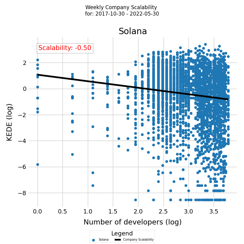
- X-axis (Log of Team Size) represents the natural logarithm of team sizes. By transforming team size to its logarithm, we're focusing on the relative changes and growth rates in team size rather than absolute changes.
- Y-axis (Log of Efficiency) represents the natural logarithm of efficiency. This transformation also emphasizes growth rates and percentage changes in efficiency.
- The line plotted through the data points is the fitted regression line, which shows the predicted relationship between the logarithm of team size and the logarithm of efficiency according to our OLS (Ordinary Least Squares) model. The slope of this line, given by the coefficient of α in our regression results, represents the elasticity of productivity with respect to team size.
The intercept in the regression output represents ln(A), and the slope represents the elasticity α of efficiency to changes in team size. We see negative values for the scaling factor α which indicate a negative relation between team size and mean efficiency (Weekly KEDE), indicating decreasing returns to scale in terms of team size.
This log-log plot and the accompanying regression analysis provide a quantitative foundation for understanding and inferring how changes in team size impact efficiency, utilizing the concept of elasticity for deeper insights into proportional relationships.
Table 1 shows the estimated coefficients of the model, inferred by means of a robust linear regression. The observed negative value for the scaling factor α = - 0.50 quantitatively confirm the negative relation between team size and mean efficiency of active developers previously observed visually in Fig. 3.
| ln(A) | Scaling Factor α | R-squared | p-value |
|---|---|---|---|
| 1.0660 | -0.4995 \(\pm\) 0.1 | 0.088 | 0.000 |
Tanle 1. MM-estimation was used to estimate the coefficient of the regressor as explained in the Appendix. The coefficient is presented together with its corresponding 95 % confidence intervals and is highly significant at p < 0.001. The sample size is 4023. The robust R2 value calculation is explained in the Appendix.
The robust R2 value of 0.0883 suggests that our model, using robust regression techniques, explains about 8.83% of the variance in the dependent variable based on the independent variables included in the model. This is a relatively low value, indicating that the model's explanatory power is modest.
In essence, our regression model allows us to infer a significant negative trend, but prevents us from making predictions about the mean efficiency, given the team size, as explained in the Appendix.
We define Scalability Coefficient as the elasticity of efficiency with respect to changes in team size, quantified as the coefficient of the log-transformed team size in a log-linear regression model.
There are three primary types of returns to scale:
- A positive Scalability Coefficient indicates that increases in team size are associated with proportional increases in efficiency, suggesting increasing returns to scale. The larger the coefficient, the stronger the positive impact of scaling up the team size on efficiency, which is beneficial for the organization.
- A constant Scalability Coefficient indicates that efficiency increases in the same proportion as team size.
- A negative Scalability Coefficient suggests that increases in team size lead to proportional decreases in efficiency, indicating decreasing returns to scale. This scenario can be problematic, implying inefficiencies where adding more developers does not translate into commensurate gains and may in fact reduce overall efficiency.
The term "Scalability Coefficient" is tailored to our specific analytical needs and context, making it relevant and directly applicable to stakeholders within your organization. It provides a clear, concise metric that can be used in strategic decision-making, planning, and discussions about scaling operations and resource allocation. By using this term within analysis or reporting, we create a benchmark for internal and external communications, facilitating clearer understanding of our analytical models and findings.
It will be a gross simplification to consider the team size alone to be the factor that drives efficiency in software development. Instead we should acknowledge that the facto is the invisible knowledge inside a team. Indeed, when we add people to an existing project the efficiency quite often decreases, as predicted by the Brooks' Law. However, it is possible to have the opposite effect and to increase efficiency just by adding the proper knowledge. As we stated several times in this article, the primary resource of software development is the knowledge in the team.
Let's look at a case where for a quite long period of 12 months a company added people and increased efficiency. Below is a time series diagram of the impact company size has had on the development capability for the period.
Along with the time series of Solana capability it's very useful to see a frequency diagram of the same data.
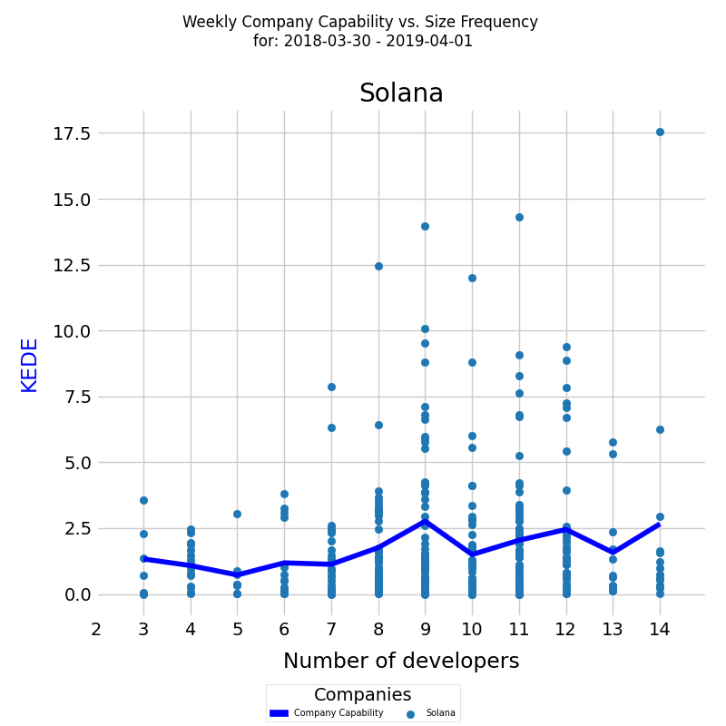
Between April and September headcount stabilized around 7. Average Efficiency increased 100%. Then from October through MAy 2019 the number of developers increased up to 14. That is a 100% increase. Efficiency also increased back to 2.5 - a 92% increase. From the frequency diagram we see that the most efficient case was when the team size was 9 developers for several weeks. We can speculate that creating and sharing of knowledge improved and efficiency increased.
On Fig. 6 we show a fitted linear regression model to understand how changes in team size are associated with changes in efficiency for all projects in a company.
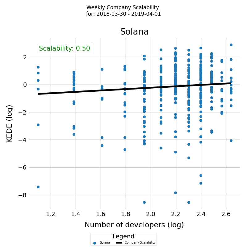
- X-axis (Log of Team Size) represents the natural logarithm of team sizes. By transforming team size to its logarithm, we're focusing on the relative changes and growth rates in team size rather than absolute changes.
- Y-axis (Log of Efficiency) represents the natural logarithm of efficiency. This transformation also emphasizes growth rates and percentage changes in efficiency.
- The line plotted through the data points is the fitted regression line, which shows the predicted relationship between the logarithm of team size and the logarithm of efficiency according to our OLS (Ordinary Least Squares) model. The slope of this line, given by the coefficient of α in our regression results, represents the elasticity of productivity with respect to team size.
Table 2 shows the estimated coefficients of the modele, inferred by means of a robust linear regression. The observed positive value for the scaling factor α = 0.5028 quantitatively confirms the positive relation between team size and mean efficiency of active developers previously observed visually in Fig. 3 for the same time period.
| ln(A) | Scaling Factor α | R-squared | p-value |
|---|---|---|---|
| -1.2389 | 0.5028 \(\pm\) 0.4 | 0.0897 | 0.017 |
Tanle 2. MM-estimation was used to estimate the coefficient of the regressor as explained in the Appendix. The coefficient is presented together with its corresponding 95 % confidence intervals and is significant at p < 0.02. The sample size is 454. The robust R2 value calculation is explained in the Appendix.
The robust R2 value of 0.0897 suggests that our model, using robust regression techniques, explains about 8.97% of the variance in the dependent variable based on the independent variables included in the model. This is a low value, indicating that the model's explanatory power is modest.
Conclusion
We have presented a methodology for measuring the scalability of software development teams based on the Knowledge Discovery Efficiency (KEDE) metric. We have shown that KEDE is a suitable measure for quantifying the efficiency of software development teams over time, providing insights into the relationship between team size and efficiency.
Our results suggest that software development teams should focus on optimizing their knowledge discovery efficiency to improve efficiency and reduce waste. By measuring and monitoring KEDE, teams can identify areas for improvement and make data-driven decisions to increase efficiency.
Overall, our methodology provides a novel approach to measuring and analyzing the scalability of software development teams, offering valuable insights into the factors that influence it.
Appendix
Calculating Robust R2 Value
The formula for calculating a type of "Robust \(R^2\)" is a conceptual adaptation of the traditional \(R^2\) calculation using median-based statistics instead of the mean[8]. This approach is not a direct implementation of any specific robust \(R^2\) formula from the literature but rather a simplified approach to achieve robustness against outliers in the calculation. Here's a breakdown of the approach:
The traditional \(R^2\) formula is:
- \(SS_{res}\) (Sum of Squared Residuals) is the sum of the squares of the residuals (differences between observed and predicted values).
- \(SS_{tot}\) (Total Sum of Squares) is the sum of the squares of the differences between observed values and their mean.
For a robust version using median-based statistics, I suggested modifying this to:
-
Robust Variance of Residuals This is calculated as the median of the absolute deviations of the residuals from their median, a robust measure of variability:
-
Robust Variance of Total Similarly, this is the median of the absolute deviations of the observed values from their median:
Inference Versus Prediction from Linear Models
Becasue KEDE values are skewed to the right and has a heavy tails or outliers, we use MM-estimation, which stands for "Maximum likelihood type estimation for the continuous part and Method of Moments for the point masses".
MM-estimation is a robust regression technique designed to provide high resistance to outliers while retaining good efficiency at the Gaussian model, making it a valuable tool in situations where data may contain anomalies or non-normal distributions that could heavily influence the results of traditional OLS regression.
We use a MM-estimation using the Robust Linear Model (RLM) from the Pthon library statsmodels.robust.robust_linear_model.RLM which can handle some aspects of robustness. The scale estimator used here is the Median Absolute Deviation (MAD), a robust measure of statistical dispersion. This differs from OLS where the scale is typically the standard deviation of the residuals. Using MAD helps reduce the influence of outliers on the scale estimation of the residuals.
In essence, our regression model allows us to infer a significant trend, but prevent us from making predictions about the mean efficiency, given the team size, as explained in the Appendix.
How to cite:
Bakardzhiev D.V. (2024) How to measure Organizational Scalability in software development. https://docs.kedehub.io/kede/kede-scalability.html
Works Cited
1. Ingo Scholtes, Pavlin Mavrodiev, and Frank Schweitzer. 2016. From Aristotle to Ringelmann: a large-scale analysis of team productivity and coordination in Open Source Software projects. Empirical Softw. Engg. 21, 2 (April 2016), 642–683. https://doi.org/10.1007/s10664-015-9406-4
2. Christoph Gote, Pavlin Mavrodiev, Frank Schweitzer, and Ingo Scholtes. 2022. Big data = big insights? operationalising brooks' law in a massive GitHub data set. In Proceedings of the 44th International Conference on Software Engineering (ICSE '22). Association for Computing Machinery, New York, NY, USA, 262–273. https://doi.org/10.1145/3510003.3510619
3. Sornette, D., Maillart, T. and Ghezzi, G., How Much Is the Whole Really More than the Sum of Its Parts? 1? 1= 2.5: Superlinear Productivity in Collective Group Actions. Plos one 9.8, e103023 (2014).
4. Ringlemann, M., Recherches sur les moteurs anim´es: Travail de l’homme, Annales de l’Institut National Agronomique. 121, (1913).
5. Brooks, F.P., The mythical man-month. Addison-Wesley (1975).
6. Bakardzhiev, D., & Vitanov, N. K. (2022). KEDE (KnowledgE Discovery Efficiency): a Measure for Quantification of the Productivity of Knowledge Workers. BGSIAM'22, p.5. Online: https://scholar.google.com/scholar?oi=bibs&hl=en&cluster=1495338308600869852
7. Bakardzhiev, D. V. (2022). U.S. Patent No. 11,372,640. Washington, DC: U.S. Patent and Trademark Office. Online: https://scholar.google.com/scholar?oi=bibs&hl=en&cluster=3749910716519444769
8. Renaud, O. and Victoria-Feser, M.-P. (2010). A robust coefficient of determination for regression, Journal of Statistical Planning and Inference 140, 1852-1862.
9. Latané, B., Williams, K.D., & Harkins, S.G. (1979). Many Hands Make Light the Work: The Causes and Consequences of Social Loafing. Journal of Personality and Social Psychology, 37, 822-832.
Getting started


